R Syntax 101: Write Your First Working Script in 10 Minutes

R's core syntax is refreshingly small. Learn five ideas, arithmetic operators, variable assignment with <-, hash comments, naming rules, and running a .R script, and you can read nearly any R code you'll ever encounter.

How do you run your first line of R code?

The fastest way to understand R is to type an expression and watch R answer back. Open RStudio, click inside the console at the bottom, and every line you type is evaluated the moment you press Enter, no compile step, no build. R is an interactive calculator that happens to also run whole scripts. Here's a three-line example that shows arithmetic, assignment, and printing in one go.

Try typing each of the four lines below. R prints the answer right under each expression that returns a value.

RArithmetic, assignment, and reuse

2 + 2 #> [1] 4 x <- 10 # store 10 in x y <- x * 3 # use x to compute y y #> [1] 30

That tiny snippet already uses three of the five syntax elements we'll cover. Line 1 is pure arithmetic: R evaluates 2 + 2 and prints 4. The strange [1] at the front is R's row index, R prints results as vectors, and [1] means "this is the first element". You can ignore it for now. Line 2 uses the <- operator to store the number 10 in a variable called x. Line 3 does the same, but reuses x in the calculation. Line 4 simply types y, and R echoes its value back.

Try it: Store your age in seconds in a variable called ex_age_seconds. A year has roughly 31,557,600 seconds.

RTry it: Age in seconds

# Try it: compute your age in seconds ex_age_seconds <- # your code here # Test: ex_age_seconds #> Expected: a large number (e.g., 946728000 for 30 years)

Click to reveal solution

RAge in seconds solution

ex_age_seconds <- 30 * 31557600 ex_age_seconds #> [1] 946728000

Explanation: Multiplying your age in years by the number of seconds in a year gives the total. Replace 30 with your own age.

Key Insight

R evaluates one line at a time, left to right, top to bottom. Every time you press Enter in the console, R reads the line, computes the result, and prints anything that wasn't assigned. Assignment silently stores the value without printing it.

What arithmetic operators does R support?

R supports seven arithmetic operators. Five of them are the usual suspects you'd find on a calculator, addition, subtraction, multiplication, division, and exponentiation. The other two are handy for integer math: modulo (remainder) and integer division. You'll use the first five constantly; the last two show up in loops, hashing, and date calculations.

Let's run every operator in a single block so you can see the results side by side.

RSeven arithmetic operators demo

5 + 2 # addition #> [1] 7 5 - 2 # subtraction #> [1] 3 5 * 2 # multiplication #> [1] 10 5 / 2 # division (always returns a decimal) #> [1] 2.5 5 ^ 2 # exponentiation (5 to the power of 2) #> [1] 25 5 %% 2 # modulo (remainder after dividing) #> [1] 1 5 %/% 2 # integer division (quotient, no remainder) #> [1] 2

Two things are worth noting. First, / in R always returns a decimal, even when both operands are whole numbers, 5 / 2 gives 2.5, not 2. If you want the integer part, use %/%. Second, ^ is the exponent operator, not **, that's a Python habit you'll have to drop.

Operator precedence in R follows standard math rules: exponentiation first, then multiplication and division, then addition and subtraction. When in doubt, use parentheses to force the order you want.

ROperator precedence with parentheses

2 + 3 * 4 # multiplication happens first #> [1] 14 (2 + 3) * 4 # parentheses override precedence #> [1] 20 2 ^ 3 + 1 # exponent first, then addition #> [1] 9

The first expression evaluates 3 * 4 = 12, then adds 2 to get 14. The second forces the addition to happen first, so you get 5 * 4 = 20. Small difference, big consequences, a stray missing parenthesis is a classic bug source in scientific code.

Tip

When in doubt, parenthesize. R does not charge extra for parentheses, and a future reader (often you, in six months) will thank you. (x - mean(x)) / sd(x) is clearer than trusting everyone to remember that division binds tighter than subtraction.

Try it: Compute the area of a rectangle that is 12.5 units wide and 8 units tall, and store it in ex_area.

RTry it: Rectangle area

# Try it: compute rectangle area ex_area <- # your code here # Test: ex_area #> Expected: 100

Click to reveal solution

RRectangle area solution

ex_area <- 12.5 * 8 ex_area #> [1] 100

Explanation: Area of a rectangle is width × height. Parentheses are unnecessary here because there's only one operation.

How do you assign values to variables in R?

A variable is a name attached to a value. Once you've stored a number, a string, or an entire dataset in a variable, you can recall it later and use it in other calculations. R has three ways to assign values, but only one is considered good style. The figure below shows the three directions side by side.

Three ways to assign values in R

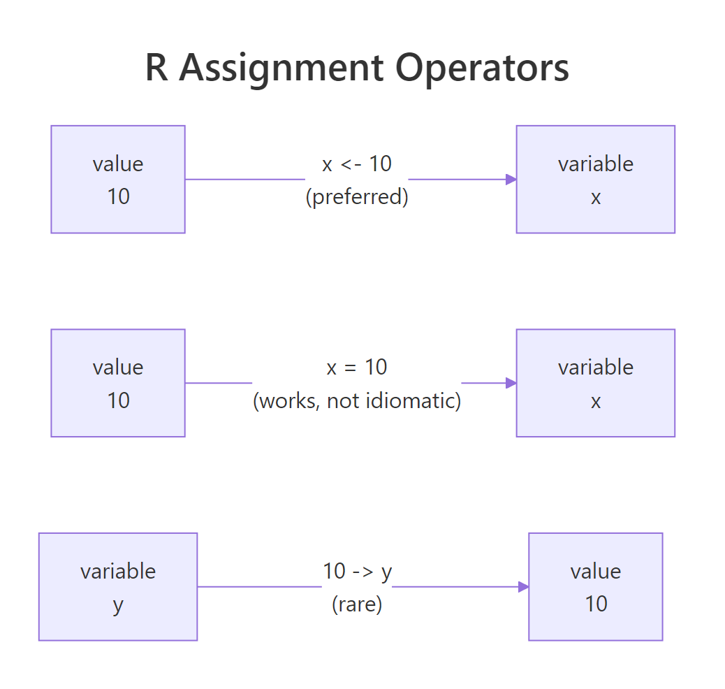
Figure 1: Three ways to assign in R, <- (idiomatic), = (valid but reserved for function arguments), and -> (rare right-to-left form).

Let's see all three operators in action. Every line below stores the number 10 in a variable, just using different syntax.

RThree ways to assign a value

a <- 10 # idiomatic left-arrow assignment b = 10 # equals-sign assignment (avoid outside function calls) 10 -> c # rare right-arrow assignment a #> [1] 10 b #> [1] 10 c #> [1] 10

All three variables now hold the same value. But even though they're functionally equivalent at the top level, the R community has overwhelmingly settled on <-. Every style guide, tidyverse, Google, Bioconductor, prefers it, so nearly all R code you'll read uses left-arrow.

Key Insight

<- and = are not identical everywhere. Inside function calls like mean(x = 1:10), the = is naming an argument, not assigning a variable. If you accidentally write <- there, R will create a new top-level variable called x as a side effect. That is why R programmers reserve = for arguments and <- for everything else, it keeps the two meanings visually separate.

You can reassign variables as often as you like. R does not complain; it just replaces the old value with the new one. Variable names are also case-sensitive, counter and Counter are two completely different variables.

RReassignment and case sensitivity

counter <- 0 counter <- counter + 1 # reassign: new value is old value + 1 counter <- counter + 1 counter #> [1] 2 Counter <- 99 # different variable, capital C Counter #> [1] 99 counter # the lowercase one is unchanged #> [1] 2

Notice how counter + 1 uses the current value of counter on the right side before the new value is assigned on the left. This "read old value, write new value" pattern is how counters and accumulators work in nearly every programming language.

Warning

Don't confuse = with ==. A single = is assignment (or argument naming). A double == is a comparison that returns TRUE or FALSE. Writing if (x = 5) when you meant if (x == 5) is a silent bug: the first assigns 5 to x and then checks whether 5 is truthy.

Try it: You have two variables ex_a <- 1 and ex_b <- 2. Swap their values using a temporary variable ex_temp, so that at the end ex_a is 2 and ex_b is 1.

RTry it: Swap two values

# Try it: swap ex_a and ex_b ex_a <- 1 ex_b <- 2 # your code here # Test: ex_a #> Expected: 2 ex_b #> Expected: 1

Click to reveal solution

RSwap variables solution

ex_a <- 1 ex_b <- 2 ex_temp <- ex_a ex_a <- ex_b ex_b <- ex_temp ex_a #> [1] 2 ex_b #> [1] 1

Explanation: You need the temporary variable because the moment you write ex_a <- ex_b, the original ex_a is lost. Save it in ex_temp first, then overwrite.

How do comments make R code readable?

A comment is a note to yourself (or the next reader) that R ignores while running the code. In R, the hash symbol # starts a comment that runs to the end of the line. Everything after the # is skipped by the interpreter. R has no multi-line comment syntax like /* ... */ in C or """...""" in Python, if you want a paragraph of explanation, put # at the start of every line.

Comments serve two purposes. First, they explain why a line exists, not what it does (the code itself already tells you what). Second, they let you temporarily disable a line of code without deleting it, which is handy when debugging.

RInline comments explain intent

# Calculate the total price including tax price <- 100 # base price in dollars tax_rate <- 0.08 # 8% sales tax # total <- price + 50 # disabled: old flat tax logic total <- price * (1 + tax_rate) total #> [1] 108

Three kinds of comments appear here. The first line is a whole-line comment explaining the block's purpose. The next two have trailing comments describing each variable. The # total <- price + 50 line is a commented-out expression, useful when you want to keep old logic around for reference or to undo a change quickly.

Tip

Write comments for the reader six months from now. "Use 0.08 because the office is in California and sales tax is 8%" is a great comment. "Set tax_rate to 0.08" is a useless one, the code already says that. Comments should explain intent, constraints, or anything that isn't obvious from the code itself.

Try it: Add a trailing comment to each line below explaining what the line does in plain English.

RTry it: Add explanatory comments

# Try it: add comments to explain each line ex_miles <- 26.2 # your comment here ex_km <- ex_miles * 1.609 # your comment here ex_km #> Expected: 42.1558

Click to reveal solution

RCommented conversion solution

ex_miles <- 26.2 # marathon distance in miles ex_km <- ex_miles * 1.609 # convert to kilometres (1 mile = 1.609 km) ex_km #> [1] 42.1558

Explanation: Good trailing comments explain units, sources, or the "why" behind a magic number, not just what the operator does.

What are the rules for naming R variables?

R is flexible about variable names, but it's not a free-for-all. A valid R name must start with a letter or a dot (.), and after that can contain letters, digits, dots, and underscores. It cannot start with a digit, cannot contain spaces or most symbols, and cannot be one of R's reserved words like TRUE, FALSE, NULL, if, or function.

RValid variable name examples

my_var <- 1 # valid: snake_case, letters and underscore userName <- 2 # valid: camelCase .hidden <- 3 # valid: leading dot (but hidden from ls()) score.1 <- 4 # valid: dots are allowed (but see note below) x2 <- 5 # valid: digits allowed after the first char my_var + userName + .hidden + score.1 + x2 #> [1] 15

All five names work, but a few would fail. 2x <- 1 is invalid because the name starts with a digit. my-var <- 1 is invalid because R reads the - as subtraction. if <- 1 is invalid because if is a reserved keyword. R will throw an "unexpected symbol" or "invalid assignment" error on any of those.

Note

Prefer snake_case for new code. The tidyverse style guide, used by most modern R packages, recommends lowercase words separated by underscores: user_name, total_sales, fit_model. Avoid dots in new variable names: my.data looks like it might be a method call on my, and historically that has caused confusion in R's S3 object system. Dots in names are valid, just not recommended.

Try it: Three of the variable names below are invalid. Rewrite them so they work and store the value on the right.

RTry it: Fix three invalid names

# Try it: fix the three invalid names # 2user <- "Alex" invalid: starts with digit # my name <- "Alex" invalid: contains a space # total$ <- 100 invalid: contains $ # your corrected code here: ex_user_name <- # ... ex_v2 <- # ... ex_total <- # ... # Test: ex_user_name #> Expected: "Alex" ex_v2 #> Expected: "Alex" ex_total #> Expected: 100

Click to reveal solution

RName fix solution

ex_user_name <- "Alex" # replaced space with underscore ex_v2 <- "Alex" # moved the digit after the letter ex_total <- 100 # dropped the $ ex_user_name #> [1] "Alex" ex_v2 #> [1] "Alex" ex_total #> [1] 100

Explanation: The fixes follow the three rules: start with a letter, no spaces, no special symbols. Underscores are the safest separator.

How do you write and run a complete R script?

Typing lines into the console is great for quick experiments, but anything you want to keep, analyses, reports, pipelines, belongs in a script file. An R script is nothing fancier than a plain text file with a .R extension that contains the same lines you'd type into the console. You save it, open it in RStudio, and run it.

How R evaluates a script

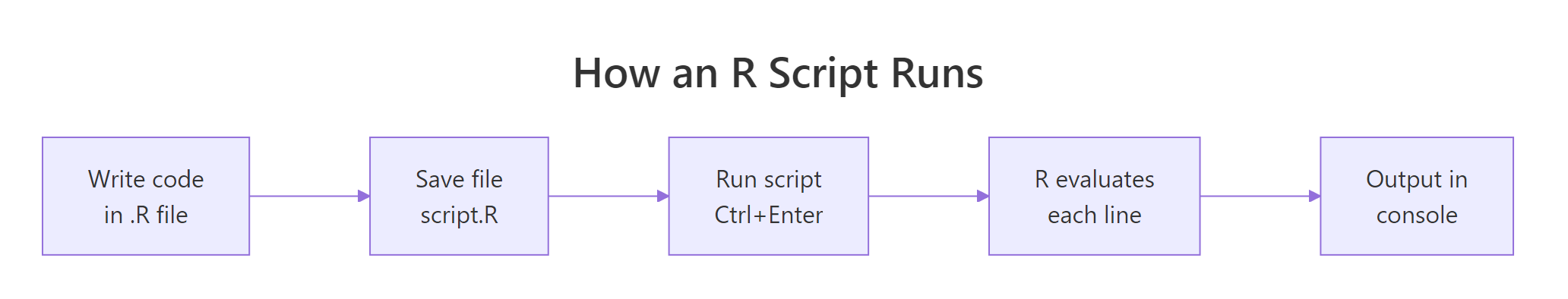
Figure 2: How R evaluates a script, write, save, run, see output. No separate compile step.

There are three common ways to run code from a script file in RStudio. You can put the cursor on any line and press Ctrl+Enter (Cmd+Enter on Mac) to run just that line. You can select several lines and press the same keys to run the selection. Or you can press Ctrl+Shift+Enter to source the entire file in one go. No matter which you pick, R evaluates the lines top to bottom in the order they appear.

Here is a complete working script you can paste into a file called temperature.R and run. It converts a Celsius temperature to Fahrenheit.

RCelsius to Fahrenheit script

# temperature.R, convert Celsius to Fahrenheit # Step 1: define the input celsius <- 25 # Step 2: apply the conversion formula F = C * 9/5 + 32 fahrenheit <- celsius * 9 / 5 + 32 # Step 3: print the result fahrenheit #> [1] 77

Read the script top to bottom. Comments mark each step so a future reader can follow along. The formula uses operator precedence: celsius * 9 / 5 is computed left to right before + 32 is added. Change celsius to any number and rerun the script, that is the core workflow of almost every R analysis you'll ever write.

Tip

Ctrl+Enter is your best friend. Running one line at a time lets you inspect intermediate results and catch mistakes early. Source the whole file only once you're confident each line works.

Try it: Modify the script so it converts kilograms to pounds instead. The conversion is pounds = kilograms * 2.20462.

RTry it: Kilograms to pounds

# Try it: kilograms to pounds kilograms <- 70 # your code here: compute and print pounds pounds <- # ... pounds #> Expected: 154.3234

Click to reveal solution

RKilograms to pounds solution

kilograms <- 70 pounds <- kilograms * 2.20462 pounds #> [1] 154.3234

Explanation: Same three-step shape as the temperature script: define the input, apply the formula, print the result. That shape will turn up in nearly every script you write.

Practice Exercises

These capstone problems combine several ideas from above. Work through them without peeking at the solutions, the struggle is where the learning happens.

Exercise 1: BMI Calculator

Write a short script that computes Body Mass Index from a person's weight (kg) and height (metres). The formula is BMI = weight / height^2. Use variables called my_weight, my_height, and my_bmi, and add comments explaining each step.

RExercise: BMI calculator

# Exercise 1: BMI calculator # Use my_weight <- 72 and my_height <- 1.75 # Hint: remember to square the height with ^ # Write your code below:

Click to reveal solution

RBMI calculator solution

# BMI calculator my_weight <- 72 # weight in kilograms my_height <- 1.75 # height in metres my_bmi <- my_weight / my_height^2 # BMI formula my_bmi #> [1] 23.51020

Explanation: The ^2 raises my_height to the power of 2, and division happens after (exponentiation binds tighter than division in R). A result around 23 puts this person in the "healthy" range on the standard BMI scale.

Exercise 2: Compound Interest

An investment of my_principal dollars grows at an annual interest rate my_rate (as a decimal, so 5% is 0.05) for my_years years. Compound-interest growth is final = principal * (1 + rate)^years. Compute the final amount for $1000 at 5% over 10 years.

RExercise: Compound interest

# Exercise 2: compound interest # Hint: use ^ for the exponent my_principal <- 1000 my_rate <- 0.05 my_years <- 10 # Compute my_final here:

Click to reveal solution

RCompound interest solution

my_principal <- 1000 my_rate <- 0.05 my_years <- 10 my_final <- my_principal * (1 + my_rate)^my_years my_final #> [1] 1628.895

Explanation: Parentheses are essential around 1 + my_rate, without them, R would compute my_rate^my_years first due to operator precedence, giving a completely wrong answer. After 10 years, $1000 grows to about $1628.89.

Exercise 3: Rectangle Analyzer

Given my_width <- 4 and my_height <- 3, compute and store three values: my_area (width × height), my_perimeter (twice the sum of width and height), and my_diagonal (the square root of width² + height², which you can compute with ^0.5).

RExercise: Rectangle area, perimeter, diagonal

# Exercise 3: rectangle analyzer my_width <- 4 my_height <- 3 # Compute my_area, my_perimeter, my_diagonal below:

Click to reveal solution

RRectangle analyzer solution

my_width <- 4 my_height <- 3 my_area <- my_width * my_height my_perimeter <- 2 * (my_width + my_height) my_diagonal <- (my_width^2 + my_height^2)^0.5 my_area #> [1] 12 my_perimeter #> [1] 14 my_diagonal #> [1] 5

Explanation: The perimeter formula needs parentheses around my_width + my_height so the addition happens before the multiplication by 2. The diagonal uses the Pythagorean theorem, and ^0.5 is a quick way to take a square root without calling sqrt(). You just computed the classic 3-4-5 right triangle.

Putting It All Together

Let's close with a complete, realistic script that uses every idea from this post in one place: a tip calculator that splits a restaurant bill. Read it top to bottom and notice how comments, assignment, arithmetic, and clear names work together.

REnd-to-end tip calculator

# tip_calculator.R, split a restaurant bill with tip # Inputs bill <- 84.50 # bill total in dollars tip_pct <- 0.18 # tip as a decimal (18%) n_people <- 4 # number of people splitting # Calculations tip_amount <- bill * tip_pct # total tip total_with_tip <- bill + tip_amount # bill + tip per_person <- total_with_tip / n_people # per-person share # Output tip_amount #> [1] 15.21 total_with_tip #> [1] 99.71 per_person #> [1] 24.9275

Every line is either a comment, a variable assignment, or a printed result. The arithmetic uses *, +, and /. The variable names are lowercase with underscores. The script runs top to bottom, with later lines reusing values computed earlier. Change any input at the top and rerun to get new answers. That is the complete mental model for writing R scripts, you now have all five syntax elements working together to solve a real problem.

Summary

The picture below is a visual recap of everything covered. Five small ideas are all it takes to read most R code.

Core R syntax elements

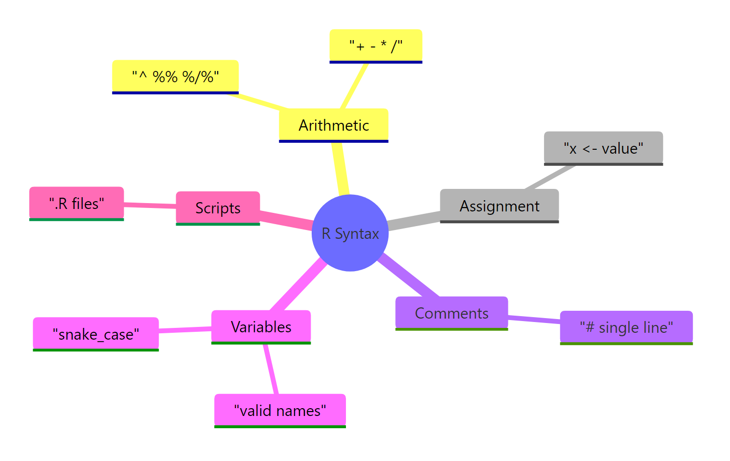
Figure 3: The five core R syntax elements covered in this post, at a glance.

Element	One-line summary	Example
Arithmetic	Seven operators: `+ - * / ^ %% %/%`	`5 + 2`, `5 ^ 2`, `5 %% 2`
Assignment	`<-` is the idiomatic way to store a value	`x <- 10`
Comments	`#` starts a comment that runs to end of line	`x <- 10 # dollars`
Naming	Start with a letter or dot; use snake_case	`my_total`, `user_name`
Scripts	A `.R` file of lines R runs top to bottom	`temperature.R` above

Master these, and the rest of R, vectors, data frames, functions, packages, is just more structure built on top. You haven't learned everything, but you've learned the grammar that everything else speaks.

References

R Core Team. An Introduction to R. CRAN. Link
R Core Team. R Language Definition. CRAN. Link
Wickham, H. Advanced R, 2nd Edition. Chapman & Hall, 2019. Chapter 2: Names and values. Link
Wickham, H. & Grolemund, G. R for Data Science, 2nd Edition. O'Reilly, 2023. Chapter 2: Workflow basics. Link
The tidyverse style guide, Syntax. Link
Posit. RStudio IDE User Guide. Link
R FAQ, CRAN. Link

Continue Learning

R Data Types, numeric, character, logical, and the other fundamental types you'll store in your newly-named variables.
R Vectors, the workhorse data structure of R. Everything you assign with <- is secretly a vector.
Writing R Functions, package the scripts you just wrote into reusable functions you can call with a single line.

{% endraw %}

R Syntax 101: Write Your First Working Script in 10 Minutes

How do you run your first line of R code?

What arithmetic operators does R support?

How do you assign values to variables in R?

How do comments make R code readable?

What are the rules for naming R variables?

How do you write and run a complete R script?

Practice Exercises

Exercise 1: BMI Calculator

Exercise 2: Compound Interest

Exercise 3: Rectangle Analyzer

Putting It All Together

Summary

References

Continue Learning

Further Reading

Related Tutorials