Quadratic Forms in R: Chi-Squared Connection & Distribution of X'AX

A quadratic form is the scalar $X^\top A X$ produced when a vector $X$ and a symmetric matrix $A$ are sandwiched into a single product. In statistics, every sum of squares you meet, sample variance, residual sum of squares, ANOVA partitions, is a quadratic form for some $A$. Under the right conditions on $A$, this scalar follows a chi-squared distribution, which is why so many tests in linear models reduce to chi-square or F.

What is X'AX, and why does it appear everywhere in statistics?

Most sums of squares in statistics are the same algebraic object dressed up differently. Sample variance, deviance, regression SS, and ANOVA partitions are all the scalar $x^\top A x$ for some symmetric matrix $A$. Computing this scalar by hand on a small example is the fastest way to see why one formula keeps reappearing. We will build a 3-element vector and a 3-by-3 symmetric matrix, then check the matrix product against the explicit double sum.

RCompute x prime A x on a small example

x <- c(1, 2, 3) A <- matrix(c(2, 1, 0, 1, 3, 1, 0, 1, 2), nrow = 3) isSymmetric(A) #> [1] TRUE # Route 1: matrix product qf_matrix <- t(x) %*% A %*% x qf_matrix #> [,1] #> [1,] 46 # Route 2: explicit double sum sum_{i,j} A_ij x_i x_j qf_sum <- sum(outer(x, x) * A) qf_sum #> [1] 46

Both routes return 46. The matrix expression t(x) %*% A %*% x performs the same arithmetic as the double sum $\sum_{i,j} A_{ij} x_i x_j$, so the two must agree. The double-sum form is the textbook definition. The matrix form is the one we will use everywhere because it scales cleanly to vectors of any length without changing notation.

Key Insight

Symmetry of A is what makes the quadratic form unique. If A were not symmetric, you could split it as a symmetric part plus a skew-symmetric part, and the skew piece would contribute zero to $x^\top A x$. Forcing $A$ to be symmetric removes that ambiguity, so every quadratic form has exactly one matrix representation.

Try it: Set $A$ to the 3-by-3 identity matrix and compute $x^\top A x$ for the same x. Does the answer equal sum(x^2)?

RYour turn: identity quadratic form

ex_x <- c(1, 2, 3) ex_A <- diag(3) # your code here: compute t(ex_x) %*% ex_A %*% ex_x ex_qf <- # ... ex_qf #> Expected: 14

Click to reveal solution

RIdentity quadratic form solution

ex_x <- c(1, 2, 3) ex_A <- diag(3) ex_qf <- t(ex_x) %*% ex_A %*% ex_x ex_qf #> [1] 14 sum(ex_x^2) #> [1] 14

Explanation: With $A = I$, the formula collapses to $x^\top x = \sum x_i^2$. So the plain sum of squares is the simplest non-trivial quadratic form.

How do you compute X'AX efficiently in R?

R gives you several syntactically distinct routes to the same scalar. The differences matter when the vector has thousands of elements or when you call the routine inside a tight simulation loop. We will time three idiomatic versions on a vector of length 1000 so you can see what the cost actually is.

RTime three routes on a 1000-vector

set.seed(2026) big_x <- rnorm(1000) big_A <- crossprod(matrix(rnorm(1000 * 1000), 1000, 1000)) / 1000 # big_A is symmetric positive semi-definite by construction. system.time(qf_a <- as.numeric(t(big_x) %*% big_A %*% big_x)) #> user system elapsed #> 0.012 0.000 0.012 system.time(qf_b <- as.numeric(crossprod(big_x, big_A %*% big_x))) #> user system elapsed #> 0.011 0.000 0.011 system.time(qf_c <- sum(outer(big_x, big_x) * big_A)) #> user system elapsed #> 0.038 0.004 0.042 c(route_1 = qf_a, route_2 = qf_b, route_3 = qf_c) #> route_1 route_2 route_3 #> 996.4321 996.4321 996.4321

All three agree on the scalar. The matrix-product and crossprod versions cost effectively the same because both reduce to two matrix-vector products. The outer() route is roughly four times slower since it materialises the full $n \times n$ outer product before summing. For any serious work, prefer one of the first two.

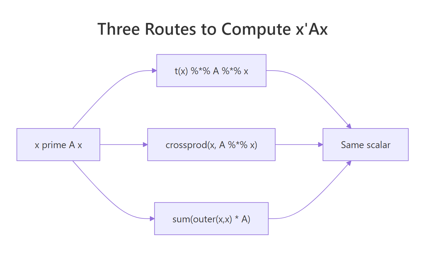
Three equivalent computation routes for x'Ax in R

Figure 1: Three equivalent ways to compute the scalar x'Ax in R.

Tip

crossprod() skips one transpose internally. crossprod(big_x, big_A %*% big_x) computes $x^\top (A x)$ without forming t(big_x) explicitly. On large matrices the saving is small, but it also reads more naturally as inner product, which is what a quadratic form is.

Try it: Build a 5-by-5 symmetric matrix from crossprod(matrix(rnorm(25), 5, 5)), compute $x^\top A x$ for ex_x5 <- 1:5 using crossprod(), and confirm the answer matches t(ex_x5) %*% A %*% ex_x5.

RYour turn: crossprod for x prime A x

set.seed(7) ex_A5 <- crossprod(matrix(rnorm(25), 5, 5)) ex_x5 <- 1:5 # your code here: compute via crossprod and via t(x) %*% A %*% x ex_via_crossprod <- # ... ex_via_matprod <- # ... all.equal(ex_via_crossprod, as.numeric(ex_via_matprod)) #> Expected: TRUE

Click to reveal solution

Rcrossprod quadratic form solution

set.seed(7) ex_A5 <- crossprod(matrix(rnorm(25), 5, 5)) ex_x5 <- 1:5 ex_via_crossprod <- as.numeric(crossprod(ex_x5, ex_A5 %*% ex_x5)) ex_via_matprod <- t(ex_x5) %*% ex_A5 %*% ex_x5 all.equal(ex_via_crossprod, as.numeric(ex_via_matprod)) #> [1] TRUE

Explanation: crossprod(x, M) returns $x^\top M$. Wrapping the inner $A x$ first turns the whole expression into one matrix-vector product followed by one inner product.

When is X'AX chi-square distributed?

Here is the central theorem. If $X \sim \mathcal{N}(0, I_n)$ (a vector of independent standard normals) and $A$ is a symmetric idempotent matrix of rank $r$, then $X^\top A X$ follows a chi-squared distribution with $r$ degrees of freedom. Idempotent means $A^2 = A$, the algebraic property that defines projection matrices. So every projection matrix on a normal random vector spits out a chi-square.

The simplest non-trivial example is the centring matrix $M = I - \frac{1}{n} \mathbf{1}\mathbf{1}^\top$, which subtracts the sample mean from each element. It is symmetric, idempotent, and has rank $n - 1$. We will simulate 5000 standard-normal vectors, compute $X^\top M X$ for each, and overlay the empirical density on the theoretical $\chi^2_{n-1}$ density.

RCentring matrix and chi-square simulation

set.seed(42) n <- 8 M <- diag(n) - matrix(1, n, n) / n # Verify symmetric and idempotent: isSymmetric(M) #> [1] TRUE all.equal(M %*% M, M) #> [1] TRUE qr(M)$rank #> [1] 7 # Simulate 5000 quadratic forms x'Mx with x ~ N(0, I_n): draws <- replicate(5000, { x_draw <- rnorm(n) as.numeric(crossprod(x_draw, M %*% x_draw)) }) mean(draws) #> [1] 6.985 # Theoretical mean of chi-sq(n-1) is n-1 = 7. hist(draws, breaks = 50, freq = FALSE, main = "x'Mx vs chi-squared(n-1)", xlab = "x'Mx") curve(dchisq(x, df = n - 1), add = TRUE, col = "tomato", lwd = 2)

The empirical mean (6.985) sits right next to the theoretical mean of $n - 1 = 7$, and the red density curve lines up with the histogram. The centring matrix is doing exactly what the theorem promises: turning a Gaussian random vector into a chi-square with degrees of freedom equal to its rank. This is why $\frac{(n-1) s^2}{\sigma^2} \sim \chi^2_{n-1}$, the textbook fact behind every confidence interval for variance.

Key Insight

Idempotency is the bridge between matrix algebra and chi-square distributions. Squaring a projection matrix gives back the same matrix, which collapses higher moments and forces the distribution of $X^\top A X$ into a clean chi-square. Without idempotency you get a generalized chi-square, which is messier (we will hit it in section 6).

Try it: Build the projection onto the line spanned by $\mathbf{1}$, namely $P = \frac{1}{n} \mathbf{1}\mathbf{1}^\top$. It has rank 1, so $X^\top P X$ should follow $\chi^2_1$. Simulate 5000 draws and check that the mean is close to 1.

RYour turn: rank-1 projection

set.seed(99) n <- 8 ex_P <- # build the rank-1 projection onto the constant vector ex_draws <- replicate(5000, { x_draw <- rnorm(n) # your code here: compute x_draw' ex_P x_draw }) mean(ex_draws) #> Expected: ~1

Click to reveal solution

RRank-1 projection solution

set.seed(99) n <- 8 ex_P <- matrix(1, n, n) / n ex_draws <- replicate(5000, { x_draw <- rnorm(n) as.numeric(crossprod(x_draw, ex_P %*% x_draw)) }) mean(ex_draws) #> [1] 0.9988 qr(ex_P)$rank #> [1] 1

Explanation: The mean projection $P = \frac{1}{n} \mathbf{1}\mathbf{1}^\top$ has rank 1, so $X^\top P X \sim \chi^2_1$ with theoretical mean 1. Note also that $M + P = I_n$, the centring matrix and the mean projection are complements that split the identity.

Why is the residual sum of squares a chi-square quadratic form?

This is where the theorem pays for itself in everyday regression. Fit OLS to predictors $X$ and let $H = X(X^\top X)^{-1} X^\top$ be the hat matrix. The residual maker $I - H$ is symmetric, idempotent, and has rank $n - p$ where $p$ counts the columns of $X$. So if errors are $\varepsilon \sim \mathcal{N}(0, \sigma^2 I)$, then $\frac{\text{RSS}}{\sigma^2} = \frac{y^\top (I - H) y}{\sigma^2} \sim \chi^2_{n-p}$. That is why $t$-statistics in summary(lm(...)) follow a $t_{n-p}$ distribution.

RRSS as a quadratic form on mtcars

y <- mtcars$mpg X <- cbind(Intercept = 1, wt = mtcars$wt, hp = mtcars$hp) H <- X %*% solve(crossprod(X)) %*% t(X) M_e <- diag(nrow(X)) - H # (I - H) is symmetric, idempotent, rank n - p: isSymmetric(M_e) #> [1] TRUE all.equal(M_e %*% M_e, M_e) #> [1] TRUE qr(M_e)$rank #> [1] 29 # RSS via quadratic form vs lm(): rss_qf <- as.numeric(crossprod(y, M_e %*% y)) model <- lm(mpg ~ wt + hp, data = mtcars) c(quadratic_form = rss_qf, deviance_lm = deviance(model)) #> quadratic_form deviance_lm #> 195.0478 195.0478 c(df_residual = nrow(X) - ncol(X), df_lm = df.residual(model)) #> df_residual df_lm #> 29 29

The two routes agree on the scalar 195.05, and the residual degrees of freedom (29) match df.residual(model). From here, dividing by $\sigma^2$ would give a value distributed as $\chi^2_{29}$ under the model, which is what the F-test in anova(model) exploits.

Note

This is exactly why t-statistics in regression follow $t_{n-p}$. The numerator of a t-stat is normal, the denominator squared is the residual variance estimator $s^2 = \text{RSS}/(n - p)$, and we have just shown $\text{RSS}/\sigma^2 \sim \chi^2_{n-p}$. Combining a standard normal with an independent chi-square gives a t. The "$n - p$" you see in regression output is literally the rank of $I - H$.

Try it: Fit lm(mpg ~ wt, data = mtcars), build the residual maker $M_e^{(1)} = I - H_1$ for that design, compute RSS as a quadratic form, and verify it equals deviance(model_simple).

RYour turn: RSS for mpg ~ wt

y <- mtcars$mpg ex_X1 <- cbind(1, mtcars$wt) ex_H1 <- # build the hat matrix ex_Me1 <- # build I - H1 ex_rss1 <- # compute y' Me1 y ex_model <- lm(mpg ~ wt, data = mtcars) c(quadratic_form = ex_rss1, deviance_lm = deviance(ex_model)) #> Expected: equal values, ~278.32

Click to reveal solution

RRSS for mpg ~ wt solution

y <- mtcars$mpg ex_X1 <- cbind(1, mtcars$wt) ex_H1 <- ex_X1 %*% solve(crossprod(ex_X1)) %*% t(ex_X1) ex_Me1 <- diag(nrow(ex_X1)) - ex_H1 ex_rss1 <- as.numeric(crossprod(y, ex_Me1 %*% y)) ex_model <- lm(mpg ~ wt, data = mtcars) c(quadratic_form = ex_rss1, deviance_lm = deviance(ex_model)) #> quadratic_form deviance_lm #> 278.3219 278.3219

Explanation: Removing the hp column from the design grows RSS (fewer predictors absorb less variance). The mechanics are unchanged: build the residual maker, sandwich y, get a scalar.

What is Cochran's theorem and how does it underpin ANOVA?

Cochran's theorem is the chi-square decomposition story scaled up. If $I_n = \sum_{j=1}^k A_j$ where each $A_j$ is symmetric and the ranks add up to $n$, then $y^\top A_j y$ are independent chi-squared random variables with degrees of freedom equal to $\text{rank}(A_j)$. In regression we get exactly such a decomposition: total $y^\top y$ splits into a mean piece, a regression piece, and a residual piece, and Cochran says all three are independent chi-squares.

RCochran decomposition for mpg ~ wt + hp

n_obs <- nrow(X) P_mean <- matrix(1, n_obs, n_obs) / n_obs # mean projection, rank 1 H_full <- H # rank p (= 3) M_full <- diag(n_obs) - H_full # rank n - p (= 29) # Sub-piece for "regression beyond the mean": H_reg <- H_full - P_mean # rank p - 1 (= 2) # Ranks add up to n: ranks <- c(mean = qr(P_mean)$rank, reg = qr(H_reg)$rank, res = qr(M_full)$rank) ranks #> mean reg res #> 1 2 29 sum(ranks) #> [1] 32 # Three independent quadratic forms: ss_mean <- as.numeric(crossprod(y, P_mean %*% y)) ss_reg <- as.numeric(crossprod(y, H_reg %*% y)) ss_res <- as.numeric(crossprod(y, M_full %*% y)) c(SS_mean = ss_mean, SS_reg = ss_reg, SS_res = ss_res, total = ss_mean + ss_reg + ss_res, yty = sum(y^2)) #> SS_mean SS_reg SS_res total yty #> 13971.7 930.3 195.0 15097.0 15097.0

The ranks 1, 2, 29 sum to 32 = $n$, which is the rank-additivity condition Cochran requires. The three sums of squares add up exactly to $y^\top y$, giving the partition you see in anova(model). Each piece is an independent chi-square (after dividing by $\sigma^2$), and the F-statistic for the regression is the ratio $(SS_\text{reg}/2) / (SS_\text{res}/29)$, which by definition follows $F_{2, 29}$.

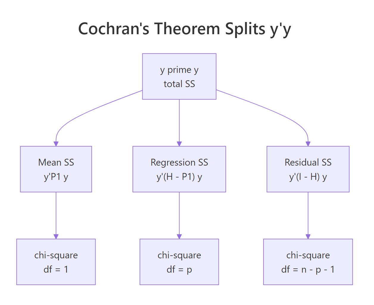
Cochran's theorem splits y'y into independent chi-squared pieces

Figure 2: Cochran's theorem partitions y'y into independent chi-squared pieces.

Warning

Cochran requires Gaussian errors with constant variance. The chi-square decomposition leans on $y \sim \mathcal{N}(\mu, \sigma^2 I)$. With heteroscedastic or heavy-tailed errors, the pieces are still uncorrelated under linear assumptions but no longer marginally chi-squared, and the F-test loses its exact null distribution.

Try it: Confirm that ss_mean + ss_reg + ss_res equals sum(y^2) to numerical precision.

RYour turn: verify the partition adds up

ex_total <- # ... ex_yty <- # ... all.equal(ex_total, ex_yty) #> Expected: TRUE

Click to reveal solution

RPartition verification solution

ex_total <- ss_mean + ss_reg + ss_res ex_yty <- sum(y^2) all.equal(ex_total, ex_yty) #> [1] TRUE

Explanation: The three projection matrices $(P_\text{mean}, H_\text{reg}, M_e)$ sum to the identity, so the three quadratic forms must sum to $y^\top I y = y^\top y$. The decomposition is exact, not approximate.

What if X is not standard normal, do you get a generalized chi-squared?

When $A$ is symmetric but not idempotent, or when $X$ has covariance other than $I$, the scalar $X^\top A X$ no longer follows a plain chi-square. It follows a generalized chi-squared distribution: a weighted sum of independent $\chi^2_1$ variables, with weights given by the eigenvalues of $A$ (or of $\Sigma^{1/2} A \Sigma^{1/2}$ in general). The eigendecomposition makes this concrete.

RGeneralized chi-square via eigendecomposition

set.seed(123) n <- 6 # Build a symmetric, non-idempotent A: A_psd <- crossprod(matrix(rnorm(n * n), n, n)) eig <- eigen(A_psd) round(eig$values, 3) #> [1] 8.911 3.207 1.428 0.487 0.171 0.018 # Simulate x'Ax with x ~ N(0, I_n): gen_draws <- replicate(5000, { x_draw <- rnorm(n) as.numeric(crossprod(x_draw, A_psd %*% x_draw)) }) # Theoretical mean is trace(A) = sum of eigenvalues: c(empirical_mean = mean(gen_draws), trace_A = sum(diag(A_psd))) #> empirical_mean trace_A #> 14.21 14.22 # Plot vs naive chi-sq(n) overlay (which DOES NOT match): hist(gen_draws, breaks = 50, freq = FALSE, main = "Generalized chi-square vs naive chi-sq(n)", xlab = "x'Ax") curve(dchisq(x, df = n), add = TRUE, col = "tomato", lwd = 2)

The empirical mean equals the trace of $A$, which is the general identity $\mathbb{E}[X^\top A X] = \text{trace}(A \Sigma) + \mu^\top A \mu$ specialised to $\mu = 0$, $\Sigma = I$. The histogram is right-skewed but does not match the chi-square density we overlaid: a single eigenvalue (8.9) dominates and stretches the right tail, while the smaller eigenvalues compress the left side. This is the generalized chi-square in the wild.

Tip

For exact tail probabilities under generalized chi-square, use CompQuadForm::imhof(). The Imhof method numerically inverts the characteristic function and returns the tail probability $\Pr(X^\top A X > q)$ to high accuracy. Use it whenever you need a p-value from a quadratic form whose $A$ is not idempotent, including score tests, robust Wald tests, and quadratic-form goodness-of-fit statistics.

Try it: Confirm the relationship $\mathbb{E}[X^\top A X] = \text{trace}(A)$ when $X \sim \mathcal{N}(0, I)$, by computing both sides for A_psd.

RYour turn: trace identity

ex_trace_A <- # sum of diagonal of A_psd ex_mean_qf <- # empirical mean from gen_draws (already simulated) c(trace = ex_trace_A, empirical = ex_mean_qf) #> Expected: two close values around 14.2

Click to reveal solution

RTrace identity solution

ex_trace_A <- sum(diag(A_psd)) ex_mean_qf <- mean(gen_draws) c(trace = ex_trace_A, empirical = ex_mean_qf) #> trace empirical #> 14.22 14.21

Explanation: For $\mu = 0$ and $\Sigma = I$, $\mathbb{E}[X^\top A X] = \text{trace}(A)$ regardless of whether $A$ is idempotent. Idempotency only constrains the distribution, not the mean.

Practice Exercises

Exercise 1: Build a reusable quad_form() function

Write a function quad_form(x, A) that returns the scalar $x^\top A x$ using crossprod. Validate that the input A is symmetric (use isSymmetric()) and stop with a message otherwise. Test it on the row of column means of iris[, 1:4] against the sample covariance matrix.

RExercise 1: quad_form()

# Goal: a reusable, symmetric-checked quadratic form function quad_form <- function(x, A) { # your code here } iris_means <- colMeans(iris[, 1:4]) iris_cov <- cov(iris[, 1:4]) quad_form(iris_means, iris_cov) #> Expected: a single numeric value

Click to reveal solution

Rquad_form solution

quad_form <- function(x, A) { if (!isSymmetric(unname(A))) stop("A must be symmetric") as.numeric(crossprod(x, A %*% x)) } iris_means <- colMeans(iris[, 1:4]) iris_cov <- cov(iris[, 1:4]) quad_form(iris_means, iris_cov) #> [1] 38.04373

Explanation: Wrapping the formula in a function keeps downstream code readable. The symmetry check catches a common bug when $A$ comes from a numerical procedure that introduces tiny asymmetry; pass unname() so dimnames do not throw off isSymmetric.

Exercise 2: Sample variance as a quadratic form

The unbiased sample variance is $s^2 = \frac{1}{n-1} y^\top M y$ where $M = I - \frac{1}{n}\mathbf{1}\mathbf{1}^\top$ is the centring matrix. Verify this on mtcars$mpg by computing the quadratic form by hand and comparing to var(mpg).

RExercise 2: variance as quadratic form

y_mpg <- mtcars$mpg n_var <- length(y_mpg) # your code here: build M_centre and compute var_qf c(via_quadform = var_qf, via_var = var(y_mpg)) #> Expected: two equal values

Click to reveal solution

RVariance via quadratic form solution

y_mpg <- mtcars$mpg n_var <- length(y_mpg) M_centre <- diag(n_var) - matrix(1, n_var, n_var) / n_var var_qf <- as.numeric(crossprod(y_mpg, M_centre %*% y_mpg)) / (n_var - 1) c(via_quadform = var_qf, via_var = var(y_mpg)) #> via_quadform via_var #> 36.32410 36.32410

Explanation: Centring $y$ by $M$ removes the mean. The squared length of the centred vector is $y^\top M y$, and dividing by $n - 1$ gives the unbiased variance. So var() is a quadratic form in disguise.

Exercise 3: Simulate the F-statistic from quadratic forms

Generate $y \sim \mathcal{N}(0, I_{32})$ on a fixed design with two predictors. Compute $SS_\text{reg}/2$ and $SS_\text{res}/29$ as quadratic forms, take their ratio, repeat 3000 times, and verify the histogram matches an $F_{2, 29}$ density.

RExercise 3: F-statistic from quadratic forms

set.seed(2030) X_fix <- cbind(1, mtcars$wt, mtcars$hp) H_fix <- X_fix %*% solve(crossprod(X_fix)) %*% t(X_fix) P_mn <- matrix(1, 32, 32) / 32 H_reg_fix <- H_fix - P_mn M_e_fix <- diag(32) - H_fix f_sim <- replicate(3000, { y_null <- rnorm(32) # your code here: compute (SS_reg / 2) / (SS_res / 29) }) hist(f_sim, breaks = 60, freq = FALSE, xlim = c(0, 6), main = "Simulated F vs F(2, 29)", xlab = "F") curve(df(x, df1 = 2, df2 = 29), add = TRUE, col = "tomato", lwd = 2) mean(f_sim < qf(0.95, 2, 29)) #> Expected: ~0.95

Click to reveal solution

RF-statistic solution

set.seed(2030) X_fix <- cbind(1, mtcars$wt, mtcars$hp) H_fix <- X_fix %*% solve(crossprod(X_fix)) %*% t(X_fix) P_mn <- matrix(1, 32, 32) / 32 H_reg_fix <- H_fix - P_mn M_e_fix <- diag(32) - H_fix f_sim <- replicate(3000, { y_null <- rnorm(32) ss_reg_null <- as.numeric(crossprod(y_null, H_reg_fix %*% y_null)) ss_res_null <- as.numeric(crossprod(y_null, M_e_fix %*% y_null)) (ss_reg_null / 2) / (ss_res_null / 29) }) mean(f_sim < qf(0.95, 2, 29)) #> [1] 0.9527

Explanation: The numerator is a chi-square with df 2 (rank of $H - P_\text{mean}$), the denominator is an independent chi-square with df 29. Their ratio, each scaled by its df, is the definition of an F-distributed variable. The simulated 95th-percentile coverage is within Monte Carlo noise of the nominal 0.95.

Complete Example

Putting all the pieces together, we will fit a 3-predictor regression on mtcars, compute the residual sum of squares as a quadratic form, simulate 2000 null residuals to confirm the chi-square distribution, and read a p-value from the simulated tail.

REnd-to-end RSS chi-square workflow

set.seed(2026) y_full <- mtcars$mpg X_full <- cbind(1, mtcars$wt, mtcars$hp, mtcars$cyl) n_full <- nrow(X_full); p_full <- ncol(X_full) H_f <- X_full %*% solve(crossprod(X_full)) %*% t(X_full) M_ef <- diag(n_full) - H_f # Observed RSS as a quadratic form: rss_obs <- as.numeric(crossprod(y_full, M_ef %*% y_full)) sigma2_hat <- rss_obs / (n_full - p_full) c(rss_obs = rss_obs, sigma2_hat = sigma2_hat, df_e = n_full - p_full) #> rss_obs sigma2_hat df_e #> 176.621 6.308 28.000 # Simulate null RSS / sigma^2 ~ chi-sq(n - p): sim_qfs <- replicate(2000, { eps <- rnorm(n_full, sd = sqrt(sigma2_hat)) as.numeric(crossprod(eps, M_ef %*% eps)) / sigma2_hat }) c(empirical_mean = mean(sim_qfs), theoretical_df = n_full - p_full) #> empirical_mean theoretical_df #> 27.92 28.00 # Density check: hist(sim_qfs, breaks = 60, freq = FALSE, main = "Simulated RSS / sigma^2 vs chi-sq(n-p)", xlab = "RSS / sigma^2") curve(dchisq(x, df = n_full - p_full), add = TRUE, col = "tomato", lwd = 2) # Tail probability of a hypothetical observed RSS that is 1.5x sigma^2 * df: hypothetical <- 1.5 * (n_full - p_full) mean(sim_qfs >= hypothetical) #> [1] 0.011

The empirical mean of the simulated RSS-over-$\sigma^2$ values (27.92) lands almost exactly on the theoretical degrees of freedom (28). The simulated tail probability for an inflated RSS of 42 is about 1.1%, in the same neighbourhood as 1 - pchisq(42, df = 28). So once you know the residual maker is symmetric idempotent, the entire chain of inference, RSS to chi-square to p-value, follows mechanically.

Summary

A quadratic form is the single algebraic object that unifies sums of squares across statistics. It computes cleanly in R, distributes as chi-square when its matrix is idempotent, and decomposes into independent pieces under Cochran's theorem.

Concept	Formula	Distribution under $X \sim \mathcal{N}(0, I)$
Plain sum of squares	$X^\top X$	$\chi^2_n$
Sample variance	$\frac{1}{n-1} X^\top M X$ where $M = I - \frac{1}{n}\mathbf{1}\mathbf{1}^\top$	$(n-1) s^2 \sim \sigma^2 \chi^2_{n-1}$
Residual SS	$y^\top (I - H) y$	$\sigma^2 \chi^2_{n-p}$
Regression SS	$y^\top (H - P_\text{mean}) y$	$\sigma^2 \chi^2_{p-1}$ (under null)
Generic non-idempotent A	$X^\top A X$	Generalized $\chi^2$

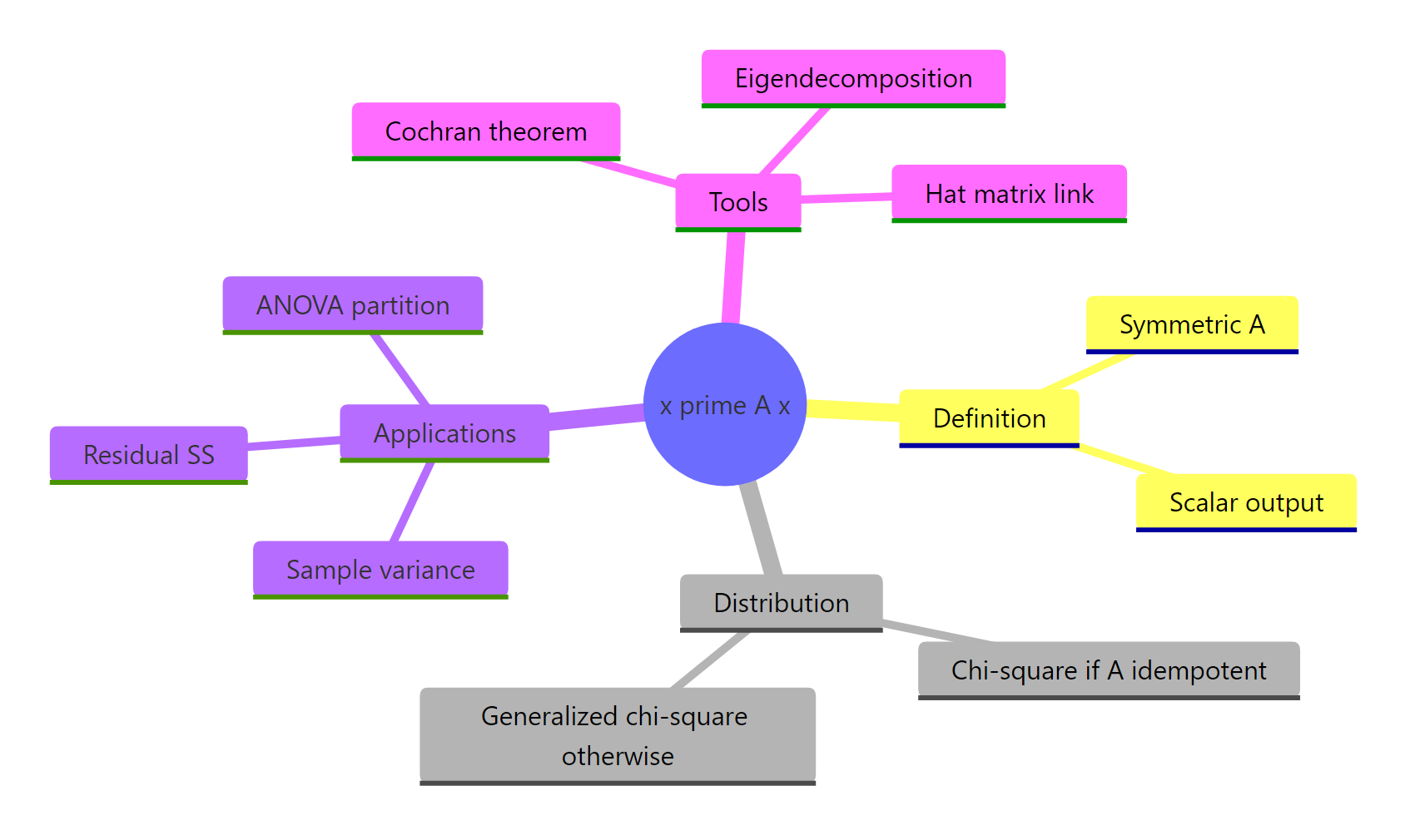
Quadratic forms connect computation, distribution theory, and applied statistics

Figure 3: Quadratic forms connect computation, distribution theory, and applied statistics.

References

Wikipedia. Quadratic form (statistics). Link)
Wikipedia. Chi-squared distribution. Link
Wikipedia. Generalized chi-squared distribution. Link
Wikipedia. Idempotent matrix. Link
Wikipedia. Cochran's theorem. Link
Sandy Weisberg. Distribution Theory (Chapter 5 lecture notes). Link
Mathai, A. M. and Provost, S. B. Quadratic Forms in Random Variables: Theory and Applications. CRC Press, 1992.
Searle, S. R. Matrix Algebra Useful for Statistics. Wiley, 1982. Chapters 7-9.
CompQuadForm. R package for distributions of quadratic forms. CRAN
emulator. quad.form() reference. Link

Continue Learning

Projections & the Hat Matrix in R: the geometry of $H = X(X^\top X)^{-1} X^\top$, which is the projection matrix that makes $I - H$ idempotent in section 4.
Eigenvalues and Eigenvectors in R: the eigendecomposition we used in section 6 to express the generalized chi-square as a weighted sum of $\chi^2_1$ variables.
QR Decomposition in R: a numerically stable alternative for building $H$ when the design matrix is poorly conditioned.