MANOVA in R: Test Multiple Outcomes Simultaneously Without Inflating Type I Error

MANOVA (Multivariate Analysis of Variance) tests whether group means differ across two or more correlated outcomes at the same time, instead of running a separate ANOVA per outcome. R's built-in manova() does it in one line. Combining outcomes into a single test controls Type I error and uncovers group differences that any single ANOVA might miss.

Why use MANOVA instead of multiple ANOVAs?

Picture three iris species and four petal-and-sepal measurements. You could fit four separate ANOVAs, but each one carries its own 5% false-positive risk. Together they balloon the family-wise error rate to roughly 19%. Worse, four solo ANOVAs ignore the correlations between the outcomes. One MANOVA solves both problems. Here is the payoff in three lines of base R.

RRun MANOVA on iris in three lines

# Test all 4 measurements vs Species in one shot iris_manova <- manova(cbind(Sepal.Length, Sepal.Width, Petal.Length, Petal.Width) ~ Species, data = iris) summary(iris_manova) #> Df Pillai approx F num Df den Df Pr(>F) #> Species 2 1.1919 53.466 8 290 < 2.2e-16 *** #> Residuals 147

Pillai's trace is 1.19, close to its theoretical maximum of k = 2 (one less than the number of groups). The approximate F is huge and the p-value is effectively zero. Translation: the three species differ on the joint pattern of all four measurements, with overwhelming evidence.

Why bother with the multivariate version? Run four ANOVAs at the standard 5% level and the chance that at least one of them gives a false positive is $1 - (1 - 0.05)^4 \approx 0.185$. That is nearly four times the nominal rate. MANOVA condenses the four tests into one, so the 5% rate stays at 5%.

Key Insight

MANOVA can detect group differences that no single ANOVA reveals. When outcomes are correlated, the cloud of group centroids in multivariate space can be far apart even when each axis alone shows weak separation. A single multivariate F sees the whole cloud at once.

Try it: Fit a smaller MANOVA on iris using just Sepal.Length and Petal.Length. Store it in ex_2dv and print the Pillai summary.

RYour turn: 2-DV MANOVA on iris

ex_2dv <- # your code here summary(ex_2dv) #> Expected: Df Pillai approx F num Df den Df Pr(>F) #> Species 2 ~0.95 ~75 ...

Click to reveal solution

RTwo-DV MANOVA solution

ex_2dv <- manova(cbind(Sepal.Length, Petal.Length) ~ Species, data = iris) summary(ex_2dv) #> Df Pillai approx F num Df den Df Pr(>F) #> Species 2 0.94895 75.728 4 294 < 2.2e-16 *** #> Residuals 147

Explanation: Trim the cbind() to two columns. Pillai drops from 1.19 to 0.95, but with two outcomes its theoretical max is also lower (1.0 here), and the test is still highly significant.

How do you run MANOVA in R with manova()?

The manova() call has the same shape as aov(). The difference lives on the left side of the formula: instead of one outcome, you bind several with cbind(). The right side is your grouping factor.

RMANOVA syntax breakdown

# Same model, but let's read every column of summary() summary(iris_manova) # default = Pillai #> Df Pillai approx F num Df den Df Pr(>F) #> Species 2 1.1919 53.466 8 290 < 2.2e-16 *** #> Residuals 147

Here is what each column means:

Df, degrees of freedom for the effect (groups − 1).
Pillai, the multivariate test statistic (R prints this one by default).
approx F, an F approximation of the statistic. MANOVA statistics do not have exact F distributions in general, so R reports an approximation that is accurate enough for inference.
num Df / den Df, the numerator and denominator degrees of freedom for that approximation.
Pr(>F), the p-value.

Note

manova() is a thin wrapper around aov() with a multivariate response. Anything you know about aov() (formulas, contrasts, factor coercion) carries over. Missing rows are dropped listwise by default; use na.omit() first if you want to be explicit.

Try it: Re-run summary() on iris_manova but ask for Wilks' lambda instead of Pillai.

RYour turn: switch to Wilks

summary(iris_manova, # your code here ) #> Expected: a Wilks column with a value around 0.02 and a similar p-value.

Click to reveal solution

RWilks lambda solution

summary(iris_manova, test = "Wilks") #> Df Wilks approx F num Df den Df Pr(>F) #> Species 2 0.023439 199.15 8 288 < 2.2e-16 *** #> Residuals 147

Explanation: Pass test = "Wilks" to summary(). Wilks' lambda is 0.023, which means roughly 2.3% of the variance in the outcome bundle is not explained by Species, so 97.7% is. Different statistic, same conclusion.

Which test statistic should you choose: Pillai, Wilks, Hotelling-Lawley, or Roy?

R's summary() prints whichever of four classical statistics you ask for. They all compress the same two matrices into a single number: the hypothesis matrix H (variation explained by the grouping factor) and the error matrix E (variation within groups). They differ in how they compress.

Statistic	Formula intuition	When to prefer
Pillai's trace	Sum of variance explained as a fraction of total	Default. Most robust to violated assumptions and unbalanced designs.
Wilks' lambda	Determinant ratio, like a multivariate $1 - R^2$	Most familiar in textbooks. Works well in balanced designs with met assumptions.
Hotelling-Lawley trace	Sum of eigenvalues of $H E^{-1}$	Slightly more powerful than Pillai when assumptions hold.
Roy's largest root	Largest eigenvalue of $H E^{-1}$	Most powerful when group means are collinear. Inflates Type I error otherwise.

Print all four side by side to see them agree on iris.

RPrint all four MANOVA statistics

# Same model, four summaries summary(iris_manova, test = "Pillai") #> Species 2 1.1919 53.466 8 290 < 2.2e-16 *** summary(iris_manova, test = "Wilks") #> Species 2 0.023439 199.15 8 288 < 2.2e-16 *** summary(iris_manova, test = "Hotelling-Lawley") #> Species 2 32.4773 580.53 8 286 < 2.2e-16 *** summary(iris_manova, test = "Roy") #> Species 2 32.1919 1167.0 4 145 < 2.2e-16 ***

The four statistics line up because the iris-versus-species effect is enormous. In real data the four can disagree at the margin, especially Roy. If three of them say significant and Roy says wildly significant, trust the others.

If you enjoy formulas, two of the cleanest definitions are:

$$\Lambda = \frac{|E|}{|H + E|} \quad\text{(Wilks)} \qquad V = \mathrm{tr}\bigl(H(H + E)^{-1}\bigr) \quad\text{(Pillai)}$$

Where:

$H$ is the between-groups sum-of-squares-and-cross-products matrix.
$E$ is the within-groups (error) matrix.
$|\cdot|$ denotes the determinant.
$\mathrm{tr}(\cdot)$ denotes the matrix trace.

If the math is not your priority, skip to the next section. The decision rules above are all you need to pick a statistic.

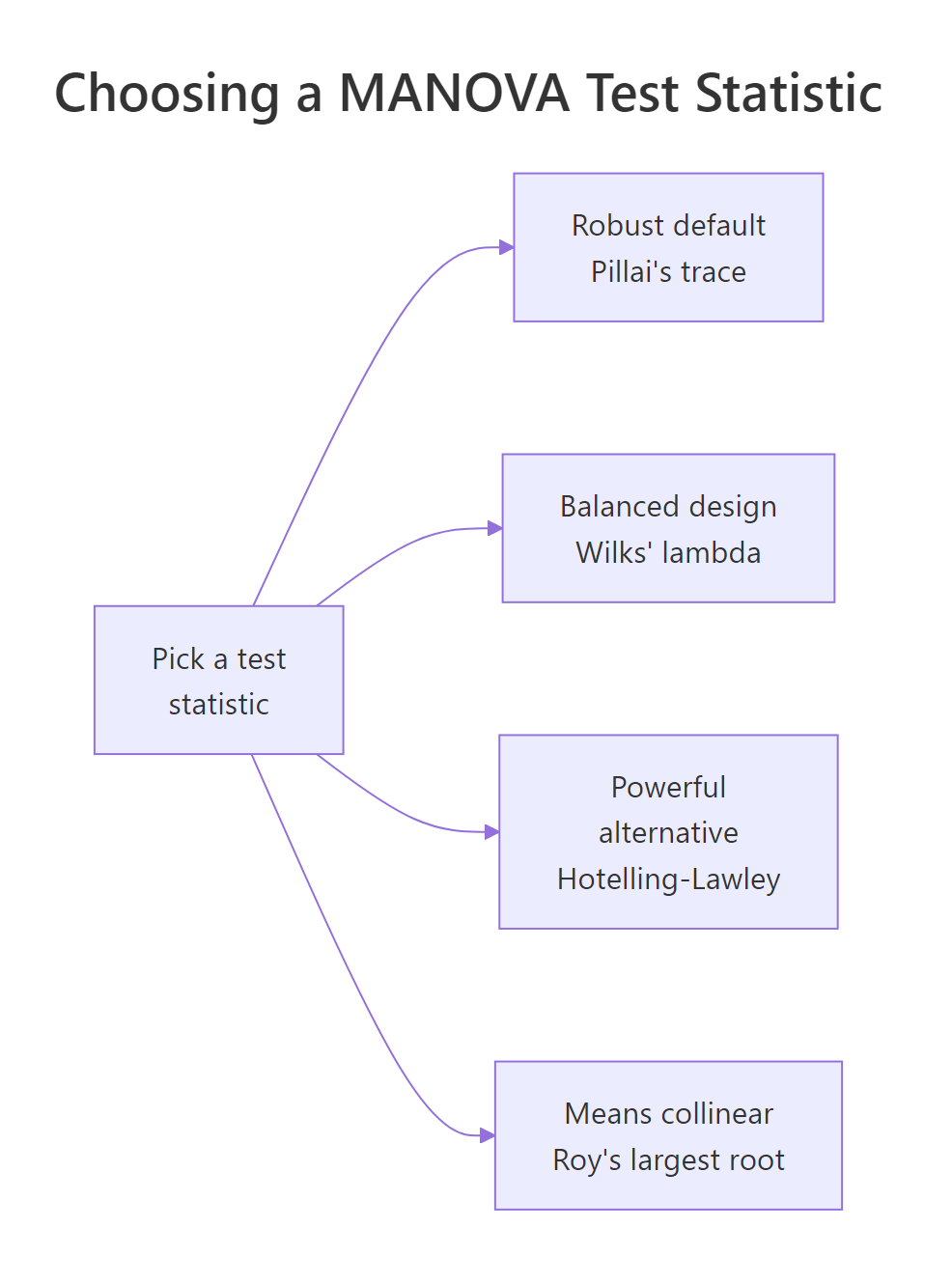
Decision flow for picking among Pillai, Wilks, Hotelling-Lawley, and Roy.

Figure 2: Picking among Pillai, Wilks, Hotelling-Lawley, and Roy.

Tip

When in doubt, report Pillai's trace. It is the safe default for unbalanced designs and mild assumption violations, which describes most real-world data. Wilks is the next-best fallback when your design is balanced.

Try it: Compute and compare Pillai and Roy on iris_manova. Note the F values.

RYour turn: Pillai vs Roy

# Print Pillai summary(iris_manova, test = # your code here ) # Print Roy summary(iris_manova, test = # your code here ) #> Expected: Pillai F approx 53, Roy F approx 1167. Both highly significant.

Click to reveal solution

RPillai vs Roy solution

summary(iris_manova, test = "Pillai") #> Species 2 1.1919 53.466 8 290 < 2.2e-16 *** summary(iris_manova, test = "Roy") #> Species 2 32.1919 1167.0 4 145 < 2.2e-16 ***

Explanation: Roy's F is roughly 22 times larger because Roy uses only the largest eigenvalue of $H E^{-1}$. Same conclusion either way, but if Roy ever stands out alone, prefer Pillai.

What assumptions does MANOVA require, and how do you check them?

MANOVA inherits ANOVA's assumptions, then adds a few because it works on a vector of outcomes. The seven things to verify:

Independence of observations, design issue, not a statistical test.
Sample size per group > number of outcomes, otherwise covariance matrices are singular.
No severe multivariate outliers, checked with Mahalanobis distance.
Multivariate normality of residuals, usually checked per outcome with Shapiro-Wilk plus QQ plots.
Equal covariance matrices across groups (homogeneity of variance-covariance), Box's M test.
No extreme multicollinearity among outcomes, drop or merge near-duplicate DVs.
Linear relationships between outcomes, scatterplot matrix per group.

Start with multicollinearity, because it is the easiest to break and the most damaging.

RCheck correlations between outcomes

# Are any DV pairs too correlated? dv_cor <- cor(iris[, 1:4]) round(dv_cor, 2) #> Sepal.Length Sepal.Width Petal.Length Petal.Width #> Sepal.Length 1.00 -0.12 0.87 0.82 #> Sepal.Width -0.12 1.00 -0.43 -0.37 #> Petal.Length 0.87 -0.43 1.00 0.96 #> Petal.Width 0.82 -0.37 0.96 1.00

Petal.Length and Petal.Width correlate at 0.96, which is in the danger zone (above 0.90 is the usual cut-off). In a real analysis you would drop one or replace both with their average. We keep both here because it does not hurt the demonstration, but be aware that two near-duplicate columns waste a degree of freedom.

Now look for multivariate outliers. Mahalanobis distance is the multivariate cousin of a z-score: it measures how far each row sits from the mean of its group, accounting for the covariance structure.

RMultivariate outliers via Mahalanobis distance

# Mahalanobis distance per row, against group mean and covariance mahal_dist <- by(iris[, 1:4], iris$Species, function(x) { mahalanobis(x, colMeans(x), cov(x)) }) # Top 3 most extreme rows per species lapply(mahal_dist, function(d) sort(d, decreasing = TRUE)[1:3]) #> $setosa #> 42 16 23 #> 17.16562 12.80317 12.40774 #> #> $versicolor #> 69 73 99 #> 11.45720 9.39250 8.92664 #> #> $virginica #> 107 132 118 #> 13.39517 9.59816 9.34366

Compare these to the chi-square critical value with k = 4 degrees of freedom: $\chi^2_{0.001, 4} \approx 18.47$. None of the top distances exceed it, so no single iris flower is wildly atypical. If you saw a value of 25 or 40, you would investigate that row before trusting the model.

Last quick check: per-outcome residual normality.

RPer-DV Shapiro-Wilk on residuals

# One Shapiro-Wilk test per outcome shapiro_results <- lapply(1:4, function(i) { shapiro.test(residuals(iris_manova)[, i]) }) sapply(shapiro_results, function(s) round(s$p.value, 4)) #> [1] 0.0500 0.1014 0.1098 0.0000

Petal.Width residuals fail Shapiro at the 5% level. With balanced designs and n = 50 per group, MANOVA tolerates mild non-normality, so this is a yellow flag, not a red one.

Warning

Box's M test for equal covariance matrices is hyper-sensitive. With large samples it almost always rejects, even when the difference between covariance matrices is trivial. Trust visual comparison of group covariance matrices, and report Pillai's trace, which is robust to mild covariance heterogeneity.

Try it: Compute the correlation matrix of mtcars columns mpg, hp, and wt. Save it to ex_cor and round to 2 decimals.

RYour turn: correlation matrix on mtcars

ex_cor <- # your code here round(ex_cor, 2) #> Expected: mpg-hp ~ -0.78, mpg-wt ~ -0.87, hp-wt ~ 0.66

Click to reveal solution

RCorrelation matrix solution

ex_cor <- cor(mtcars[, c("mpg", "hp", "wt")]) round(ex_cor, 2) #> mpg hp wt #> mpg 1.00 -0.78 -0.87 #> hp -0.78 1.00 0.66 #> wt -0.87 0.66 1.00

Explanation: cor() returns a symmetric matrix. Subset the columns first, then round for readability. None of the pairs cross the 0.90 multicollinearity threshold.

How do you follow up a significant MANOVA?

A significant Pillai answers "yes, groups differ on the joint outcome bundle." It does not say which outcomes drive the difference, and it does not say which groups differ. Two follow-up steps close the loop.

The first step is summary.aov(), which prints a univariate ANOVA per outcome from the same model object. No re-fitting needed.

RUnivariate ANOVA per outcome

# Run one ANOVA per outcome, all from the MANOVA model summary.aov(iris_manova) #> Response Sepal.Length : #> Df Sum Sq Mean Sq F value Pr(>F) #> Species 2 63.212 31.606 119.26 < 2.2e-16 *** #> #> Response Sepal.Width : #> Df Sum Sq Mean Sq F value Pr(>F) #> Species 2 11.345 5.6725 49.16 < 2.2e-16 *** #> #> Response Petal.Length : #> Df Sum Sq Mean Sq F value Pr(>F) #> Species 2 437.10 218.55 1180.2 < 2.2e-16 *** #> #> Response Petal.Width : #> Df Sum Sq Mean Sq F value Pr(>F) #> Species 2 80.41 40.205 960.01 < 2.2e-16 ***

All four outcomes are significant on their own, but the F values rank them: Petal.Length (F = 1180) and Petal.Width (F = 960) drive the species difference far more than the sepal measurements. With four follow-up tests, apply a Bonferroni correction: divide your alpha by k. At $\alpha = 0.05$ and k = 4, the per-test threshold becomes 0.0125. All four still pass.

Second step: pairwise comparisons within the strongest outcome. TukeyHSD() controls the family-wise error rate across the three species pairs.

RPairwise comparisons on the strongest outcome

# TukeyHSD needs a univariate aov() model tukey_petal <- TukeyHSD(aov(Petal.Length ~ Species, data = iris)) tukey_petal #> $Species #> diff lwr upr p adj #> versicolor-setosa 2.798 2.5942 3.0018 0 #> virginica-setosa 4.090 3.8862 4.2938 0 #> virginica-versicolor 1.292 1.0882 1.4958 0

All three pairwise differences in Petal.Length are significant. The largest gap (4.09 cm) sits between setosa and virginica, the smallest (1.29 cm) between versicolor and virginica. That gives you the full story: species differ jointly, the petal measurements drive most of it, and every species pair is distinguishable.

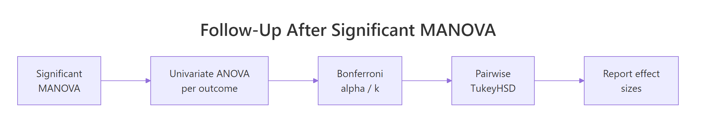
Workflow after a significant MANOVA: univariate ANOVA per outcome, Bonferroni adjustment, pairwise contrasts.

Figure 3: Follow-up workflow after a significant multivariate F test.

Note

The effectsize and emmeans packages offer richer post-hoc tools, but they are not available in this in-browser session. The base-R recipes above run anywhere. For partial eta squared by hand: $\eta^2_p = \mathrm{SS}_\mathrm{effect} / (\mathrm{SS}_\mathrm{effect} + \mathrm{SS}_\mathrm{error})$, computed from each row of summary.aov() output.

Try it: Look back at the summary.aov(iris_manova) output. Which outcome has the largest F value for Species, and roughly what is its F?

Click to reveal solution

Petal.Length has the largest F at 1180.2. Petal.Width is second at 960. The two sepal measurements lag well behind. In a write-up you would highlight petal length as the dominant driver of the species difference.

How do you run a two-way MANOVA with interactions?

Real designs often have two factors. The same manova() call handles them, you just put both factors on the right side joined with * for an interaction.

RTwo-way MANOVA on mtcars

# Two factors: cylinders and transmission. Two outcomes: mpg and hp. mt_manova <- manova(cbind(mpg, hp) ~ factor(cyl) * factor(am), data = mtcars) summary(mt_manova) #> Df Pillai approx F num Df den Df Pr(>F) #> factor(cyl) 2 1.06425 17.7196 4 52 1.066e-08 *** #> factor(am) 1 0.32341 5.9799 2 25 0.007621 ** #> factor(cyl):factor(am) 2 0.36888 2.8635 4 52 0.032076 * #> Residuals 26

Read it row by row. The main effect of cyl is hugely significant: cylinder count moves the (mpg, hp) joint outcome. The main effect of am (transmission) is also significant. The interaction row is significant at the 5% level too, which means the effect of transmission on the (mpg, hp) bundle depends on cylinder count. In other words, the gap between automatic and manual cars is not the same in 4-cylinder, 6-cylinder, and 8-cylinder cars.

Note

Two-way MANOVA in base R uses Type I (sequential) sums of squares. When your design is unbalanced, the order of factors in the formula affects the main-effect tests. For Type III tests (each effect adjusted for all others), use car::Manova() in a local R session. The car package is not available in the in-browser sandbox.

Try it: Re-fit the same two-way MANOVA but with only main effects (no interaction). Save it to ex_main.

RYour turn: main-effects-only two-way MANOVA

ex_main <- # your code here summary(ex_main) #> Expected: factor(cyl) ~ Pillai 1.07, factor(am) ~ Pillai 0.32, both significant.

Click to reveal solution

RMain-effects MANOVA solution

ex_main <- manova(cbind(mpg, hp) ~ factor(cyl) + factor(am), data = mtcars) summary(ex_main) #> Df Pillai approx F num Df den Df Pr(>F) #> factor(cyl) 2 1.06425 17.7196 4 56 4.046e-09 *** #> factor(am) 1 0.32341 5.9799 2 27 0.006996 ** #> Residuals 28

Explanation: Replace * with + to drop the interaction. The two main effects keep the same Pillai values but get more denominator degrees of freedom (28 vs 26 residuals), which slightly tightens the p-values.

Practice Exercises

Exercise 1: MANOVA on airquality

Use the built-in airquality data. Treat Month as the grouping factor. Use cbind(Ozone, Solar.R, Wind, Temp) as the joint outcome. The dataset has missing values, so drop incomplete rows first with na.omit(). Fit MANOVA, request Wilks' lambda, then call summary.aov() and identify the outcome with the largest F. Save the model as aq_manova.

RExercise: airquality MANOVA

# Hint: na.omit() first, then manova(cbind(...) ~ Month, data = ...) # Hint: Coerce Month to factor or it will be treated as numeric. # Write your code below:

Click to reveal solution

Rairquality MANOVA solution

aq <- na.omit(airquality) aq_manova <- manova(cbind(Ozone, Solar.R, Wind, Temp) ~ factor(Month), data = aq) summary(aq_manova, test = "Wilks") #> Df Wilks approx F num Df den Df Pr(>F) #> factor(Month) 4 0.32988 5.7368 16 324.55 9.392e-12 *** #> Residuals 106 summary.aov(aq_manova) #> Response Ozone : F = 11.22, p = 1.6e-07 #> Response Solar.R: F = 1.69, p = 0.157 #> Response Wind : F = 3.83, p = 0.006 #> Response Temp : F = 41.06, p < 2.2e-16

Explanation: Temp has the largest F (41), so monthly temperature differences drive most of the joint effect. Solar.R is the only outcome that is not individually significant after Bonferroni at $0.05/4 = 0.0125$.

Exercise 2: Compare all four statistics in one tidy table

Build a single data frame called stat_table with one row per test statistic (Pillai, Wilks, Hotelling-Lawley, Roy), holding the statistic value, the approximate F, and the p-value for the Species effect of iris_manova. Use summary() with each test = option and pull the numbers out of the returned object.

RExercise: tidy table of all four statistics

# Hint: summary(iris_manova, test = "Pillai")$stats holds the numbers. # Hint: stats is a matrix; the Species row is row 1. # Write your code below:

Click to reveal solution

RAll-four-statistics table solution

tests <- c("Pillai", "Wilks", "Hotelling-Lawley", "Roy") stat_table <- do.call(rbind, lapply(tests, function(t) { s <- summary(iris_manova, test = t)$stats data.frame(test = t, statistic = round(s["Species", 2], 4), approx_F = round(s["Species", "approx F"], 2), p_value = signif(s["Species", "Pr(>F)"], 3)) })) stat_table #> test statistic approx_F p_value #> 1 Pillai 1.1919 53.47 0 #> 2 Wilks 0.0234 199.15 0 #> 3 Hotelling-Lawley 32.4773 580.53 0 #> 4 Roy 32.1919 1167.00 0

Explanation: summary(...)$stats is a numeric matrix; column 2 is always the statistic value regardless of which one you asked for. All four agree that Species matters, but Roy's F dwarfs the others, a reminder that Roy is the most aggressive of the four.

Complete Example

Putting the full workflow on iris end to end:

RComplete MANOVA workflow on iris

# 1. Inspect table(iris$Species) #> setosa versicolor virginica #> 50 50 50 # 2. Check correlations among outcomes round(cor(iris[, 1:4]), 2) #> (matrix from earlier; Petal.Length-Petal.Width = 0.96) # 3. Fit MANOVA iris_full <- manova(cbind(Sepal.Length, Sepal.Width, Petal.Length, Petal.Width) ~ Species, data = iris) # 4. Pillai summary (default, robust) summary(iris_full) #> Species 2 1.1919 53.466 8 290 < 2.2e-16 *** # 5. Per-outcome ANOVAs summary.aov(iris_full) #> Sepal.Length F=119, Sepal.Width F=49 #> Petal.Length F=1180, Petal.Width F=960 # 6. Pairwise comparisons on the strongest outcome TukeyHSD(aov(Petal.Length ~ Species, data = iris)) #> All three pairs significant; biggest gap virginica vs setosa (4.09 cm).

Plain-English conclusion: the three iris species differ jointly on the four floral measurements (Pillai = 1.19, F(8, 290) = 53.5, p < 0.001). Petal length and petal width drive most of the difference, and every species pair is distinguishable on petal length, with the virginica-setosa gap the largest. That sentence is exactly the kind of write-up a journal expects.

Summary

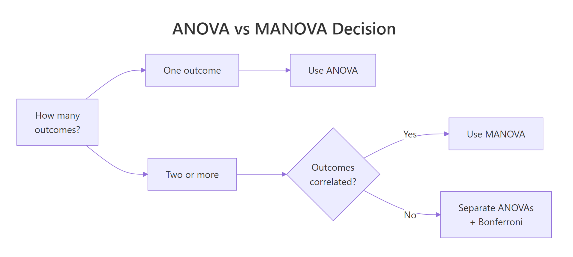
Decision flow for choosing between ANOVA, multiple ANOVAs with Bonferroni, and MANOVA.

Figure 1: Decision flow for choosing between ANOVA, multiple ANOVAs with Bonferroni, and MANOVA.

Idea	Takeaway
Why MANOVA	Tests k correlated outcomes in one shot; controls family-wise Type I error.
Syntax	`manova(cbind(y1, y2, ...) ~ x, data = df)`
Default statistic	Pillai's trace, printed by `summary()`.
Robust default	Pillai is best when assumptions wobble or the design is unbalanced.
Risky statistic	Roy's largest root over-rejects unless group means are collinear.
Assumption to fear most	Multicollinearity among outcomes (cor > 0.9).
First follow-up	`summary.aov()` for univariate ANOVA per outcome, with Bonferroni alpha = 0.05/k.
Second follow-up	`TukeyHSD()` on the strongest outcome for pairwise contrasts.
Two-way design	Same call, just `factor1 * factor2` on the right of `~`.

References

Wilks, S. S. (1932). Certain generalizations in the analysis of variance. Biometrika, 24(3-4), 471-494.
Bartlett, M. S. (1939). A note on tests of significance in multivariate analysis. Mathematical Proceedings of the Cambridge Philosophical Society, 35(2), 180-185.
R Core Team. ?manova and ?summary.manova in base R. Link
Fox, J., & Weisberg, S. (2019). An R Companion to Applied Regression, 3rd ed. Sage. (Chapter on multivariate linear models and car::Manova().)
Tabachnick, B. G., & Fidell, L. S. (2019). Using Multivariate Statistics, 7th ed. Pearson. Chapter 7 on MANOVA.
Hand, D. J., & Taylor, C. C. (1987). Multivariate Analysis of Variance and Repeated Measures. Chapman & Hall.
Penn State STAT 505. Lesson 8.3: Test Statistics for MANOVA. Link
STHDA. MANOVA Test in R: Multivariate Analysis of Variance. Link

Continue Learning

One-Way ANOVA in R, the single-outcome version that MANOVA generalises. Read this first if the F-table feels unfamiliar.
Two-Way ANOVA in R, what the two-factor case looks like with a single outcome. Useful contrast for the two-way MANOVA section above.
Post-Hoc Tests After ANOVA, deeper coverage of TukeyHSD(), Bonferroni, and pairwise contrasts you will use after summary.aov().