Chi-Square Test of Independence in R: Assumptions, Effect Size & Power

The chi-square test of independence checks whether two categorical variables are related in a population by comparing the counts you observe in a contingency table to the counts you'd expect if the variables were independent. Most tutorials stop at the p-value; this one walks the full pipeline, assumption checks, effect size with Cramer's V, and a power analysis you can run on your own data.

What does the chi-square test of independence actually answer?

Suppose you have survey data with two categorical columns, say smoking status and exercise level, and you want to know whether they move together or are unrelated. The chi-square test of independence answers exactly this. It compares the counts you actually observed against the counts you would expect if the two variables had nothing to do with each other, then turns the gap into a single p-value. Let's run one now.

RRun the chi-square test on real survey data

library(MASS) # Build a 2-way contingency table from the survey dataset tbl <- table(survey$Smoke, survey$Exer) tbl #> Freq None Some #> Heavy 7 1 3 #> Never 87 18 84 #> Occas 12 3 4 #> Regul 9 1 7 # Test whether smoking status and exercise level are independent xt <- chisq.test(tbl) xt #> #> Pearson's Chi-squared test #> #> data: tbl #> X-squared = 5.4885, df = 6, p-value = 0.4828

You ran the test in two lines. The chi-square statistic is 5.49 with 6 degrees of freedom, and the p-value is 0.48. Because the p-value is well above any standard threshold (0.05, 0.01), you do not reject the null hypothesis of independence. In plain language: smoking status and exercise level look unrelated in this sample.

Note

The test detects association, not causation. A small p-value tells you the two variables move together more than chance would predict. It does not say one causes the other, or in which direction.

Try it: Run the same test on survey$Smoke against survey$Sex to check whether smoking varies by sex in this dataset. Save the fitted test to ex_xt.

RYour turn: smoking by sex

# Try it: build the table and run the test ex_tbl <- # your code here ex_xt <- # your code here # Print: ex_xt #> Expected: a chisq.test result with X-squared, df, and p-value

Click to reveal solution

RSmoking by sex solution

ex_tbl <- table(survey$Smoke, survey$Sex) ex_xt <- chisq.test(ex_tbl) ex_xt #> #> Pearson's Chi-squared test #> #> data: ex_tbl #> X-squared = 0.5418, df = 3, p-value = 0.9095

Explanation: table() cross-tabulates the two factors, then chisq.test() does the rest. The high p-value here (0.91) means smoking patterns look similar across sexes in this sample.

How do you check the assumptions before trusting the result?

Three assumptions sit underneath every chi-square test of independence, and skipping the checks is the single most common mistake practitioners make. Let's walk them.

Independent observations. Each count in the table comes from a separate, independent unit (one row per person, one survey response per person). Repeated measures or matched pairs break this assumption, you'd use McNemar's test instead.
Expected counts large enough. Every cell's expected count should be at least 5. A common relaxation: at most 20% of cells may have expected counts below 5, and no cell should have expected count below 1.
Fixed categories with random sampling. Categories are defined before data collection, and rows of the dataset are a random sample of the population.

The first and third are study-design questions. The second is something you must verify from R every single time.

RInspect expected counts and the small-cell rule

# Pull the matrix of expected counts under the null exp_counts <- xt$expected round(exp_counts, 1) #> Freq None Some #> Heavy 5.4 1.0 4.6 #> Never 65.4 12.5 56.1 #> Occas 8.2 1.6 7.2 #> Regul 6.0 1.1 5.9 # How many cells have expected count < 5? low_cells <- sum(exp_counts < 5) total_cells <- length(exp_counts) prop_low <- low_cells / total_cells c(low_cells = low_cells, total = total_cells, proportion = round(prop_low, 2)) #> low_cells total proportion #> 6.00 12.00 0.50

Half the cells have expected counts below 5, and several cells (Heavy/None, Occas/None, Regul/None) have expected counts of 1 or below. This breaks the rule of thumb. Treat the p-value with suspicion until you re-run the test with a method that handles small expected counts (covered later in the Yates / simulate / Fisher section).

When the assumption is badly violated, R itself often warns you. Let's reproduce the warning on a clearly small table.

RReproduce the small-expected-count warning

# Construct a 2x3 table where some expected counts are tiny small_tbl <- matrix(c(2, 1, 8, 1, 2, 9), nrow = 2, byrow = TRUE, dimnames = list(group = c("A", "B"), response = c("X", "Y", "Z"))) small_tbl #> response #> group X Y Z #> A 2 1 8 #> B 1 2 9 chisq.test(small_tbl) #> Warning message: #> In chisq.test(small_tbl): Chi-squared approximation may be incorrect #> #> Pearson's Chi-squared test #> #> data: small_tbl #> X-squared = 0.6957, df = 2, p-value = 0.7062

The warning Chi-squared approximation may be incorrect is R's way of telling you the asymptotic p-value cannot be trusted. It is not optional. Ignoring it can flip a significant result to non-significant or vice versa.

Warning

Never report a chi-square p-value while ignoring the small-expected-count warning. The p-value is computed from a continuous chi-square distribution, but with sparse cells the actual sampling distribution is jagged and discrete. The two diverge, so your p-value is wrong, sometimes badly.

Try it: Write ex_check_expected(tbl) that returns TRUE if at least 80% of cells have expected count >= 5 AND no cell has expected count below 1. Test it on tbl from earlier and on small_tbl.

RYour turn: assumption checker

ex_check_expected <- function(tbl) { # your code here } # Test on both: ex_check_expected(tbl) ex_check_expected(small_tbl) #> Expected: FALSE for both (tbl has too many low cells; small_tbl has cells <1 too)

Click to reveal solution

RAssumption checker solution

ex_check_expected <- function(tbl) { e <- chisq.test(tbl)$expected prop_ok <- mean(e >= 5) no_tiny <- all(e >= 1) prop_ok >= 0.80 & no_tiny } ex_check_expected(tbl) #> [1] FALSE ex_check_expected(small_tbl) #> [1] FALSE

Explanation: chisq.test(tbl)$expected returns the expected-count matrix without you having to recompute it. mean(e >= 5) is the share of cells meeting the floor, and all(e >= 1) enforces the absolute minimum. Both must hold.

What do the chi-square statistic, p-value, and degrees of freedom mean?

Once the assumptions hold, the three numbers in the output have specific roles:

Chi-square statistic ($\chi^2$) measures how far observed counts sit from expected counts, summed across all cells. Bigger means more departure from independence.
Degrees of freedom (df) is (rows - 1) * (cols - 1). It captures the number of cells in the table that are free to vary once the row and column totals are fixed.
p-value is the probability of seeing a chi-square statistic at least as extreme as yours if the null (independence) were true.

The formula is small enough to read in one line:

$$\chi^2 = \sum_{i,j} \frac{(O_{ij} - E_{ij})^2}{E_{ij}}$$

Where:

$O_{ij}$ = observed count in row $i$, column $j$
$E_{ij}$ = expected count under independence: $\frac{\text{row}_i \text{ total} \times \text{col}_j \text{ total}}{\text{grand total}}$
The sum runs over every cell in the table.

That's it, no fitting algorithm, no iteration. Pull the components from the fitted object to see the math directly.

RExtract test components

# All four pieces in one go list( statistic = xt$statistic, df = xt$parameter, p_value = xt$p.value ) #> $statistic #> X-squared #> 5.48848 #> #> $df #> df #> 6 #> #> $p_value #> [1] 0.4828415 # Pearson residuals: (O - E) / sqrt(E) per cell round(xt$residuals, 2) #> Freq None Some #> Heavy 0.69 -0.01 -0.74 #> Never 2.67 1.55 3.74 #> Occas 1.34 1.11 -1.18 #> Regul 1.21 -0.13 0.45

Pearson residuals turn the global statistic into a per-cell story. A residual near 0 means that cell behaved as expected; a large positive residual means more observations landed there than expected; a large negative one means fewer. The biggest values flag where the action is.

For tighter tail probabilities, use standardized residuals. They have approximate variance 1, so values outside |2| are roughly the chi-square equivalent of a 5%-level z-score.

RStandardized residuals to localize the association

round(xt$stdres, 2) #> Freq None Some #> Heavy 0.84 -0.01 -1.00 #> Never 0.83 0.96 -1.49 #> Occas 1.66 1.27 -1.42 #> Regul 1.49 -0.15 0.55 # Find the cell with the largest absolute standardized residual which(abs(xt$stdres) == max(abs(xt$stdres)), arr.ind = TRUE) #> row col #> Occas 3 1

The largest standardized residual is in the Occas/Freq cell, but at 1.66 it does not exceed |2|, consistent with the non-significant overall test. If you ever see a standardized residual of 3 or 4 in a non-significant test, double-check, you may have an interaction worth investigating.

Key Insight

The omnibus test answers whether an association exists; residuals tell you where it lives. A significant chi-square with all small residuals is suspicious; a non-significant chi-square with one giant residual is suspicious in the other direction. Always look at both.

Try it: From xt, extract the row name and column name of the cell with the highest absolute standardized residual. Save them to ex_row and ex_col.

RYour turn: locate the strongest cell

idx <- # your code here ex_row <- # your code here ex_col <- # your code here c(row = ex_row, col = ex_col) #> Expected: row="Occas", col="Freq"

Click to reveal solution

RLocate the strongest cell solution

idx <- which(abs(xt$stdres) == max(abs(xt$stdres)), arr.ind = TRUE) ex_row <- rownames(xt$stdres)[idx[1, "row"]] ex_col <- colnames(xt$stdres)[idx[1, "col"]] c(row = ex_row, col = ex_col) #> row col #> "Occas" "Freq"

Explanation: which(..., arr.ind = TRUE) returns row/column indices for matrix entries; you then look up the names from rownames() and colnames() of the residual matrix.

How big is the effect? Computing Cramer's V, phi, and contingency coefficient

The p-value answers "is the association real?". With 50,000 observations, even a tiny, practically meaningless association will return a p-value below 0.001. Effect size answers "is the association big enough to care about?". For r-by-c tables, the standard measure is Cramer's V.

$$V = \sqrt{\frac{\chi^2}{n \cdot \min(r-1, c-1)}}$$

Where:

$\chi^2$ = the chi-square statistic from the test
$n$ = total sample size (sum of all cells)
$r$, $c$ = number of rows and columns in the table.

V ranges from 0 (no association) to 1 (perfect association). For 2x2 tables, V reduces to the phi coefficient, which is just $\sqrt{\chi^2 / n}$. The math is simple enough that you do not need a separate package, base R will do it.

RCompute Cramer's V from the fitted test

# Pull the pieces chi2 <- as.numeric(xt$statistic) n <- sum(tbl) r <- nrow(tbl) c <- ncol(tbl) # Cramer's V v_cramer <- sqrt(chi2 / (n * min(r - 1, c - 1))) round(v_cramer, 3) #> [1] 0.097 # Phi (only meaningful for 2x2 tables, shown for comparison) phi <- sqrt(chi2 / n) round(phi, 3) #> [1] 0.137

Cramer's V of 0.10 is tiny. The chi-square test gave us p = 0.48 and now we know that even if it were significant, the practical association would be negligible.

The interpretation thresholds depend on the smaller dimension of the table. Cohen's commonly cited cutoffs are below.

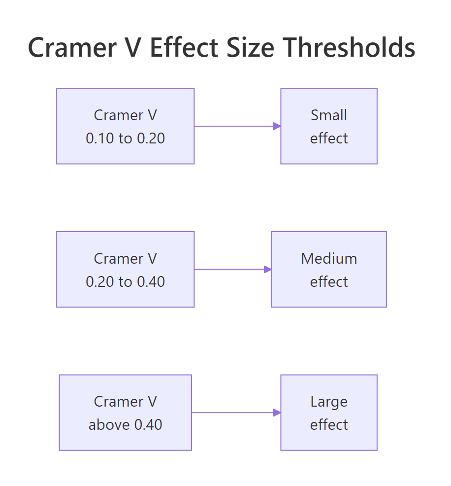
Cramer's V interpretation thresholds for small, medium, and large effects.

Figure 1: Cramer's V interpretation thresholds for small, medium, and large effects.

df = min(r-1, c-1)	Small	Medium	Large
1 (2x2 table)	0.10	0.30	0.50
2 (e.g. 2x3, 3x3)	0.07	0.21	0.35
3 (e.g. 2x4, 4x4)	0.06	0.17	0.29
4	0.05	0.15	0.25

Use these as guidelines, not laws. A V of 0.12 is "small" by Cohen but might be the most important finding in your study, depending on context.

Tip

Always report effect size alongside the p-value. Statistical significance is a function of n; practical significance is what your reader cares about. A reviewer who sees only p < 0.001 and no V is reading half the result.

Try it: Compute Cramer's V manually for ex_xt (the smoking-by-sex test you ran earlier). The total sample size is sum(ex_tbl). Save your answer to ex_v.

RYour turn: compute Cramer's V

ex_chi2 <- # your code here ex_n <- # your code here ex_r <- # your code here ex_c <- # your code here ex_v <- # your code here round(ex_v, 3) #> Expected: a small value near 0.05 (smoking and sex are barely associated here)

Click to reveal solution

RCramer's V solution

ex_chi2 <- as.numeric(ex_xt$statistic) ex_n <- sum(ex_tbl) ex_r <- nrow(ex_tbl) ex_c <- ncol(ex_tbl) ex_v <- sqrt(ex_chi2 / (ex_n * min(ex_r - 1, ex_c - 1))) round(ex_v, 3) #> [1] 0.048

Explanation: as.numeric() strips the named-vector wrapper from $statistic so the arithmetic stays clean. The min(r-1, c-1) term is what makes V comparable across tables of different shapes.

When should you use Yates correction, simulate.p.value, or switch to Fisher's exact?

R's default behavior changes with table size, and the choice of correction affects your p-value. Three knobs are worth knowing.

For 2x2 tables, chisq.test() applies the Yates continuity correction by default. This subtracts 0.5 from each |O - E| before squaring, which makes the test more conservative (bigger p-values). For larger tables, Yates does not apply.

For tables with sparse cells, you have two robust choices: Monte Carlo simulation of the p-value, or Fisher's exact test.

RYates correction on vs. off (2x2 table)

# A 2x2 example: did people pass or fail by treatment group tbl_2x2 <- matrix(c(20, 30, 35, 15), nrow = 2, byrow = TRUE, dimnames = list(group = c("Treatment", "Control"), outcome = c("Pass", "Fail"))) tbl_2x2 #> outcome #> group Pass Fail #> Treatment 20 30 #> Control 35 15 xt_yates_on <- chisq.test(tbl_2x2) # default: correct = TRUE xt_yates_off <- chisq.test(tbl_2x2, correct = FALSE) c(yates_on = xt_yates_on$p.value, yates_off = xt_yates_off$p.value) #> yates_on yates_off #> 0.005140391 0.002770340

Yates pushes the p-value from 0.0028 to 0.0051, a meaningful shift near common decision thresholds. Statisticians have argued for decades over whether Yates is appropriate; modern practice is split. If you are unsure, reporting both is honest.

Note

Yates only applies to 2x2 tables. For 3x3 or larger, R ignores correct even if you set it. Many older tutorials do not mention this and produce confusing output for newcomers.

When expected counts are too small, neither correction will fix the issue. Switch to a method that does not rely on the chi-square approximation at all.

RSparse cells: simulate p-value and Fisher's exact

# small_tbl from earlier had cells with expected counts near 1 # Option A: Monte Carlo p-value (works on any table size) set.seed(2026) xt_sim <- chisq.test(small_tbl, simulate.p.value = TRUE, B = 10000) xt_sim #> #> Pearson's Chi-squared test with simulated p-value (based on 10000 replicates) #> #> data: small_tbl #> X-squared = 0.6957, df = NA, p-value = 0.7868 # Option B: Fisher's exact test (computes the exact p-value) fisher.test(small_tbl) #> #> Fisher's Exact Test for Count Data #> #> data: small_tbl #> p-value = 0.7748 #> alternative hypothesis: two.sided

Both give p-values around 0.78, very close to each other and well above 0.05. Either would be a defensible report; Fisher's is preferred for 2x2 tables and small overall samples (n < 20-30), while Monte Carlo scales better to larger sparse tables.

The decision tree below summarizes the choice.

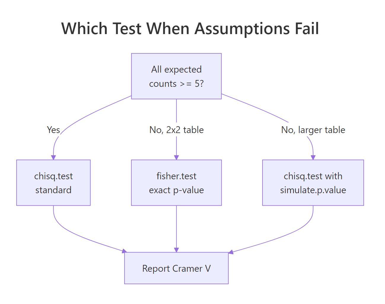
Decision tree: which test or correction to use when assumptions are violated.

Figure 2: Decision tree for picking between standard chi-square, simulated p-value, and Fisher's exact.

Try it: You have a 2x2 table where one expected count is below 5. Run the appropriate test (hint: it is in the diagram above) and save the resulting p-value to ex_p.

RYour turn: pick the right test

ex_tbl_small <- matrix(c(8, 2, 3, 1), nrow = 2, byrow = TRUE, dimnames = list(group = c("A", "B"), outcome = c("Yes", "No"))) # Check expected counts first: chisq.test(ex_tbl_small)$expected #> outcome #> group Yes No #> A 7.857143 2.142857 #> B 3.142857 0.857143 <- below 5 (and below 1) # Pick and run the right test: ex_p <- # your code here ex_p #> Expected: a p-value near 1.0 (no association; very small sample)

Click to reveal solution

RRight test for sparse 2x2 solution

ex_p <- fisher.test(ex_tbl_small)$p.value ex_p #> [1] 1

Explanation: With a 2x2 table and an expected count below 1, neither standard chi-square nor Yates fixes the problem. Fisher's exact uses the hypergeometric distribution to compute an exact p-value, no asymptotic approximation involved.

How do you compute statistical power and required sample size?

Power analysis answers two related questions:

Post-hoc: Given my sample size, what effect size could I have detected with 80% power?
A-priori: To detect an effect of a given size with 80% power, how big a sample do I need?

The chi-square test's power depends on the sample size $n$, degrees of freedom $df$, the alpha level, and the effect size $w$, which is a population analog of Cramer's V (small = 0.10, medium = 0.30, large = 0.50 for df = 1). The math uses the noncentral chi-square distribution. The popular helper for this is pwr::pwr.chisq.test(), but the underlying computation is two lines of base R via pchisq(), which is what we'll show here.

RPost-hoc power: what could you detect with n you have?

# Reuse the survey contingency table: n = 235, df = 6 n_obs <- sum(tbl) # 235 df_test <- (nrow(tbl) - 1) * (ncol(tbl) - 1) # 6 alpha <- 0.05 # Power for a "small" effect (w = 0.10) with this n and df w <- 0.10 ncp <- (w^2) * n_obs # noncentrality parameter crit_value <- qchisq(1 - alpha, df_test) # critical chi-square at alpha power <- 1 - pchisq(crit_value, df_test, ncp = ncp) round(power, 3) #> [1] 0.169 # Repeat for medium (w = 0.30) and large (w = 0.50) for (eff in c(0.10, 0.30, 0.50)) { ncp_e <- (eff^2) * n_obs pw <- 1 - pchisq(crit_value, df_test, ncp = ncp_e) cat("w =", eff, " power =", round(pw, 3), "\n") } #> w = 0.1 power = 0.169 #> w = 0.3 power = 0.954 #> w = 0.5 power = 1

With n = 235 and df = 6, you have only 17% power to detect a small effect (w = 0.10). The non-significant result you saw earlier could just mean your study was underpowered, not that the effect doesn't exist. For a medium effect you have 95% power, that finding is trustworthy.

To turn the question around, find the smallest n that gives 80% power. Solve numerically with a small loop.

RA-priori sample size for 80% power

# Target: how many observations needed for 80% power, w = 0.30, df = 2, alpha = 0.05? target_power <- 0.80 w_target <- 0.30 df_target <- 2 alpha <- 0.05 crit <- qchisq(1 - alpha, df_target) # Walk n upward until power crosses target for (n in seq(10, 500, by = 1)) { ncp_n <- (w_target^2) * n pw <- 1 - pchisq(crit, df_target, ncp = ncp_n) if (pw >= target_power) { n_required <- n break } } n_required #> [1] 107

You need 107 observations to detect a medium effect (w = 0.30) on a df = 2 table with 80% power at alpha = 0.05. This is the kind of number you'd report in a grant application or pre-registration document.

Tip

Run the a-priori power analysis BEFORE collecting data, not after. Post-hoc power computed from the observed effect size is mathematically tied to the p-value and tells you nothing new. The useful question is always: "for the effect size I would care about, was my sample big enough?", which is an a-priori question.

Try it: Compute the sample size needed for w = 0.25, df = 4, alpha = 0.01, and power = 0.90. Save the answer to ex_n.

RYour turn: a-priori sample size

ex_w <- 0.25 ex_df <- 4 ex_alpha <- 0.01 ex_target <- 0.90 ex_crit <- # your code here ex_n <- NA for (n in seq(10, 1000, by = 1)) { # your code here } ex_n #> Expected: an integer near 300 (smaller effect + stricter alpha + higher power = bigger n)

Click to reveal solution

RA-priori sample size solution

ex_w <- 0.25 ex_df <- 4 ex_alpha <- 0.01 ex_target <- 0.90 ex_crit <- qchisq(1 - ex_alpha, ex_df) ex_n <- NA for (n in seq(10, 1000, by = 1)) { ncp_n <- (ex_w^2) * n pw <- 1 - pchisq(ex_crit, ex_df, ncp = ncp_n) if (pw >= ex_target) { ex_n <- n break } } ex_n #> [1] 313

Explanation: Stricter alpha (0.01 vs 0.05), higher target power (0.90 vs 0.80), and a smaller effect size (0.25 vs 0.30) all push n upward. 313 is what each of those constraints demands together.

Practice Exercises

These capstone exercises combine the steps above. Use distinct variable names (my_*) so they don't collide with the tutorial's notebook state.

Exercise 1: Sex and smoking, end-to-end

Using MASS::survey, test whether Sex and Smoke are independent. Report the chi-square statistic, df, and p-value, then compute Cramer's V. Save Cramer's V to my_v_sex_smoke.

RExercise 1 starter

# Hint: build the table, run chisq.test(), then plug into the V formula. my_tbl_ss <- # your code here # Continue:

Click to reveal solution

RExercise 1 solution

my_tbl_ss <- table(survey$Sex, survey$Smoke) my_xt_ss <- chisq.test(my_tbl_ss) my_xt_ss #> Pearson's Chi-squared test #> data: my_tbl_ss #> X-squared = 0.5418, df = 3, p-value = 0.9095 my_chi2 <- as.numeric(my_xt_ss$statistic) my_n <- sum(my_tbl_ss) my_v_sex_smoke <- sqrt(my_chi2 / (my_n * min(nrow(my_tbl_ss) - 1, ncol(my_tbl_ss) - 1))) round(my_v_sex_smoke, 3) #> [1] 0.048

Explanation: A p-value of 0.91 plus V of 0.05 means there is essentially no relationship between sex and smoking in this dataset, a clear "no" on every dimension.

Exercise 2: Sparse 2x2, three different p-values

Build the 2x2 table below, where one expected count drops below 5. Run three tests: standard chisq.test() (Yates on), chisq.test(simulate.p.value = TRUE), and fisher.test(). Save the three p-values to my_p_chi, my_p_sim, and my_p_fisher. Which is most defensible to report?

RExercise 2 starter

my_sparse <- matrix(c(12, 2, 3, 4), nrow = 2, byrow = TRUE, dimnames = list(arm = c("Drug", "Placebo"), response = c("Recovered", "Did not"))) # Run all three tests my_p_chi <- # your code here my_p_sim <- # your code here my_p_fisher <- # your code here c(chi = my_p_chi, sim = my_p_sim, fisher = my_p_fisher)

Click to reveal solution

RExercise 2 solution

set.seed(7) my_p_chi <- chisq.test(my_sparse)$p.value # warning expected my_p_sim <- chisq.test(my_sparse, simulate.p.value = TRUE, B = 20000)$p.value my_p_fisher <- fisher.test(my_sparse)$p.value c(chi = my_p_chi, sim = my_p_sim, fisher = my_p_fisher) #> chi sim fisher #> 0.04534878 0.05344733 0.05633398

Explanation: The standard chi-square crosses 0.05 (looks "significant") but the warning fires. Simulated and Fisher both sit just above 0.05 and agree with each other. Fisher is most defensible here, exact, no approximation, and standard for sparse 2x2 tables.

Exercise 3: Sample size for a pilot

A pilot study estimated w = 0.25 (small-to-medium) on a contingency table with df = 4. You want 90% power at alpha = 0.01 for the main study. How many observations do you need? Save to my_n.

RExercise 3 starter

# Hint: same loop pattern as the a-priori example in the power section, # just plug in different values. my_n <- # your code here my_n

Click to reveal solution

RExercise 3 solution

my_w <- 0.25 my_df <- 4 my_alpha <- 0.01 my_target <- 0.90 my_crit <- qchisq(1 - my_alpha, my_df) my_n <- NA for (n in seq(10, 1000, by = 1)) { pw <- 1 - pchisq(my_crit, my_df, ncp = (my_w^2) * n) if (pw >= my_target) { my_n <- n; break } } my_n #> [1] 313

Explanation: Same answer (313) as the inline exercise, the harder constraints on alpha and power matter more than the slightly larger df.

Complete Example

Here is the full pipeline on a different dataset, HairEyeColor, a 3-way array shipped with base R. We'll collapse over Sex, run the full test, and write a publishable summary.

REnd-to-end: hair color and eye color

# Step 1: aggregate to a 2-way table (collapse the Sex dimension) he_tbl <- apply(HairEyeColor, c(1, 2), sum) he_tbl #> Eye #> Hair Brown Blue Hazel Green #> Black 68 20 15 5 #> Brown 119 84 54 29 #> Red 26 17 14 14 #> Blond 7 94 10 16 # Step 2: assumption check he_test <- chisq.test(he_tbl) mean(he_test$expected >= 5) # share of cells passing the rule of thumb #> [1] 1 all(he_test$expected >= 1) #> [1] TRUE # Step 3: run the test he_test #> #> Pearson's Chi-squared test #> #> data: he_tbl #> X-squared = 138.29, df = 9, p-value < 2.2e-16 # Step 4: localize the association via standardized residuals round(he_test$stdres, 1) #> Eye #> Hair Brown Blue Hazel Green #> Black 8.4 -5.9 0.2 -2.7 #> Brown 5.1 -6.2 2.7 -0.4 #> Red -1.0 -3.4 1.7 3.6 #> Blond -10.5 14.2 -3.0 2.9 # Step 5: effect size he_chi2 <- as.numeric(he_test$statistic) he_n <- sum(he_tbl) he_v <- sqrt(he_chi2 / (he_n * min(nrow(he_tbl) - 1, ncol(he_tbl) - 1))) round(he_v, 3) #> [1] 0.279 # Step 6: power for a medium effect at this sample size and df he_df <- (nrow(he_tbl) - 1) * (ncol(he_tbl) - 1) he_crit <- qchisq(0.95, he_df) he_pwr <- 1 - pchisq(he_crit, he_df, ncp = (0.30^2) * he_n) round(he_pwr, 3) #> [1] 1

Reportable summary (3 sentences):

A chi-square test of independence found a strong association between hair color and eye color, $\chi^2$(9, N = 592) = 138.3, p < .001. Cramer's V = 0.28, a medium-to-large effect. Standardized residuals show the largest deviations among Blond hair: substantially fewer brown-eyed (z = -10.5) and substantially more blue-eyed (z = 14.2) blondes than independence would predict.

That paragraph is the deliverable, statistic, df, n, p-value, effect size, and a sentence locating the association. It is what every reviewer wants to see.

Summary

The chi-square test of independence is a six-step pipeline, not a one-line call.

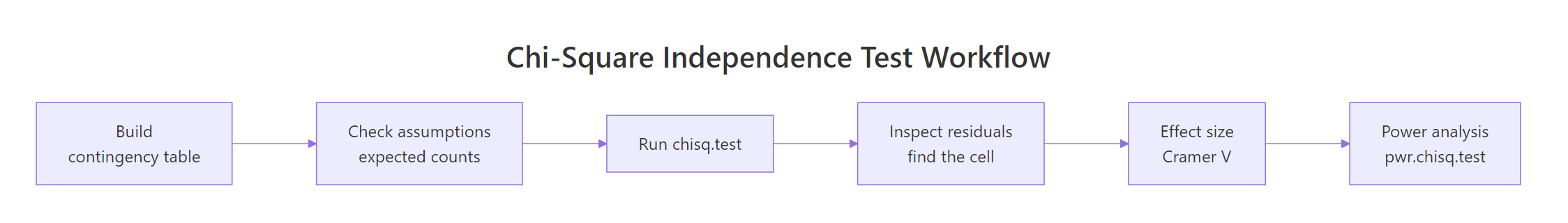
The full chi-square workflow, from contingency table to power analysis.

Figure 3: The full chi-square workflow, from contingency table to power analysis.

Step	What to do	R function
1. Build table	Cross-tab the two categorical variables	`table()`
2. Check assumptions	Verify expected counts >= 5 in 80%+ of cells	`chisq.test()$expected`
3. Run test	Compute $\chi^2$, df, p-value	`chisq.test()`
4. Locate effect	Inspect standardized residuals	`chisq.test()$stdres`
5. Effect size	Compute Cramer's V	$\sqrt{\chi^2 / (n \cdot \min(r-1, c-1))}$
6. Power	Post-hoc detection or a-priori sample size	`pchisq()` with ncp
Fallbacks	Sparse table	`simulate.p.value` or `fisher.test()`

Three habits separate good practice from p-value chasing: always inspect expected counts, always report effect size, and run an a-priori power analysis before collecting data.

References

R Core Team. chisq.test: Pearson's Chi-squared Test for Count Data. R documentation. Link
Cohen, J. (1988). Statistical Power Analysis for the Behavioral Sciences, 2nd ed. Lawrence Erlbaum Associates.
Agresti, A. (2018). An Introduction to Categorical Data Analysis, 3rd ed. Wiley.
Champely, S. The pwr package: Basic functions for power analysis. CRAN. Link
Yates, F. (1934). Contingency tables involving small numbers and the chi-square test. Journal of the Royal Statistical Society Supplement, 1(2), 217-235.
Cramer, H. (1946). Mathematical Methods of Statistics. Princeton University Press.
McHugh, M. L. (2013). The chi-square test of independence. Biochemia Medica, 23(2), 143-149. Link

Continue Learning

Categorical Data in R: Frequency Tables, Crosstabs & Mosaic Plots, the foundation post on building contingency tables, mosaic plots, and reading proportions before you ever run a test.
Chi-Square Goodness-of-Fit Test in R, the sister test, asking whether one categorical variable matches an expected distribution rather than asking whether two variables are related.
Fisher's Exact Test in R, go deeper on the exact-test alternative recommended for sparse 2x2 tables.

Chi-Square Test of Independence in R: Assumptions, Effect Size & Power

What does the chi-square test of independence actually answer?

How do you check the assumptions before trusting the result?

What do the chi-square statistic, p-value, and degrees of freedom mean?

How big is the effect? Computing Cramer's V, phi, and contingency coefficient

When should you use Yates correction, simulate.p.value, or switch to Fisher's exact?

How do you compute statistical power and required sample size?

Practice Exercises

Exercise 1: Sex and smoking, end-to-end

Exercise 2: Sparse 2x2, three different p-values

Exercise 3: Sample size for a pilot

Complete Example

Summary

References

Continue Learning

Related Tutorials