McNemar's Test in R: Paired Categorical Data & Matched Case-Control
McNemar's test compares two paired proportions on the same subjects. It looks only at the cells where two paired measurements disagree (the discordant pairs) and asks whether one direction of change is more common than the other. Reach for it whenever the same person, item, or matched pair contributes both data points.
What problem does McNemar's test solve?
Suppose 794 voters watch a debate and you record their preferred candidate before and after. A regular chi-square test cannot answer "did opinions shift?" here, because each voter contributes two linked observations and chi-square assumes those rows are independent. McNemar's test fixes this by ignoring everyone whose answer stayed the same, and asking whether the people who changed moved mostly in one direction. Let's run it.
The test ignores the 48 voters who picked A both times and the 510 who picked B both times. It only counts the 150 who switched A to B and the 86 who switched B to A. The chi-square value is 16.8 with one degree of freedom and a p-value near zero, so the asymmetry between 150 and 86 is far larger than chance would explain. Net opinion moved toward candidate B.
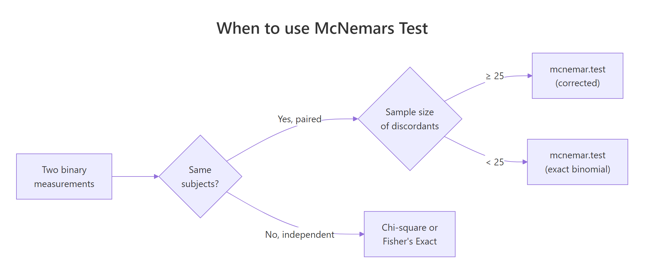
Figure 1: Decision flow: choosing between McNemar, chi-square, and the exact binomial form.
Try it: Swap the two discordant counts (86 and 150) so the directions are equal. Predict what the p-value should be, then run it.
Click to reveal solution
Explanation: When b == c, the numerator (b - c)^2 is zero, so the chi-square statistic is zero and the p-value is 1. There is no evidence of asymmetric change.
How does the discordant-pair logic work?
Every paired 2x2 table has four cells: a and d are the concordant pairs (both measurements agree), while b and c are the discordant pairs (the measurements disagree, in opposite directions). McNemar's test only uses b and c. The intuition is simple: if there is no real shift between the two timepoints, a subject who did change is equally likely to have moved in either direction, so we expect b and c to be roughly equal.
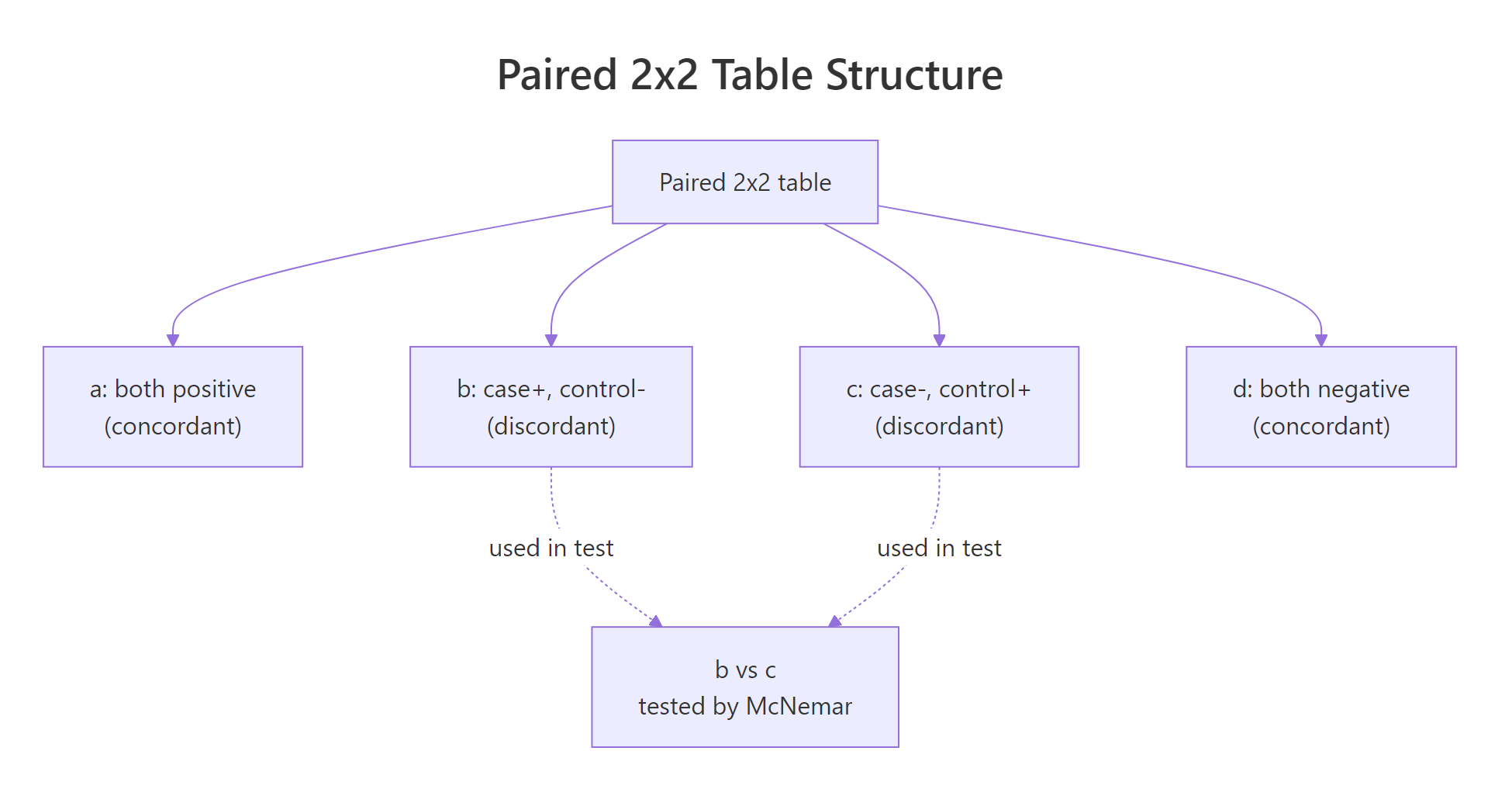
Figure 2: Anatomy of the paired 2x2 table, only the discordant cells (b, c) drive the test.
The test statistic itself is short:
$$\chi^2 = \frac{(b - c)^2}{b + c}$$
Where:
- $b$ = pairs that went from "yes" to "no" (or first category to second)
- $c$ = pairs that went from "no" to "yes"
- $\chi^2$ follows a chi-square distribution with 1 degree of freedom under H0
Let's compute the statistic by hand and compare it with mcnemar.test() (with correct = FALSE, so R uses the same formula).
The two numbers match, which confirms the formula and confirms that mcnemar.test() ignores the concordant cells entirely. The p-value drops slightly versus the corrected version we ran above because we removed the continuity correction.
Try it: Compute the McNemar chi-square by hand for b = 12 and c = 4, then verify with mcnemar.test() on a 2x2 matrix where the concordant cells can be anything (set them to 100 each).
Click to reveal solution
Explanation: The concordant counts (100, 100) do not affect the statistic at all, only b and c do.
How does the continuity correction change the result?
By default, mcnemar.test() applies a Yates-style continuity correction: it subtracts 1 from |b - c| before squaring. This nudges the p-value upward to compensate for using a continuous chi-square distribution to approximate a discrete count statistic. With large discordant totals the correction barely moves the answer; with small ones it can flip a borderline result.
Both p-values are tiny here, so the conclusion does not change. But notice how the corrected statistic is smaller and the p-value is larger. That extra padding is doing exactly what it claims: making the test slightly more conservative.
correct = TRUE for routine reporting. It matches the behavior most reviewers and textbooks expect. Switch to correct = FALSE only when you want the raw formula or are comparing against a hand calculation.Try it: Compare corrected vs uncorrected on the small table b = 12, c = 4 from the last exercise (use ex_tab). Which p-value is larger?
Click to reveal solution
Explanation: With only 16 discordant pairs, the correction pushes the p-value from 0.046 to 0.080, crossing the conventional 0.05 threshold. This is exactly the regime where you should think about an exact test instead.
When should you use the exact binomial version?
When the total number of discordant pairs b + c is small, the chi-square approximation is unreliable. A common rule of thumb is to use the exact form whenever b + c < 25. The exact McNemar test is just a binomial test in disguise: under the null hypothesis, each discordant pair is equally likely to flip in either direction, so b follows a Binomial(b + c, 0.5) distribution. We can run this directly with binom.test().
The exact p-value is 0.0768, which lands between the continuity-corrected (0.0801) and uncorrected (0.0455) chi-square versions, and is the most trustworthy of the three when discordant pairs are this scarce. With only 16 discordant pairs, you should report the exact p-value instead of the chi-square one.
b + c < 25. The chi-square distribution is a poor approximation for so few discordant pairs. The exact binomial p-value above is the safe choice, and it costs you nothing extra.Try it: Run an exact McNemar on b = 1, c = 7. What does the p-value say?
Click to reveal solution
Explanation: Only 8 discordant pairs is firmly in exact-test territory. The p-value of 0.07 says the imbalance (1 vs 7) is not quite significant at the conventional 5 percent threshold, even though the proportion looks lopsided.
How do you run McNemar's test on a matched case-control study?
In a 1:1 matched case-control study, every case is paired with one control matched on age, sex, and other confounders. You then ask whether the case was exposed to a risk factor more often than its matched control. The 2x2 table cross-classifies exposure (yes/no) for case versus control. Concordant pairs (both exposed, or both not exposed) carry no information about the case-control difference. Discordant pairs do all the work, and the matched odds ratio is simply b / c.
Twenty pairs had a smoking case with a non-smoking control, while only 5 pairs had the reverse. McNemar's p-value of 0.005 says this asymmetry is unlikely under the null. The matched odds ratio of 4 means a case is four times as likely to be the exposed member of the pair, suggesting smoking is associated with lung cancer in this matched design.
Try it: What is the matched OR if you flip the discordant cells (so b = 5 and c = 20)?
Click to reveal solution
Explanation: Flipping the direction inverts the odds ratio. An OR of 0.25 says the exposed member of the pair is less likely to be the case, which would suggest a protective effect.
What if your table is bigger than 2x2?
mcnemar.test() also accepts square k x k tables, where it tests marginal homogeneity: whether the row totals and column totals come from the same distribution. This is useful for ordinal scales, like a rater's 3-level score before and after training. For larger tables R uses the Stuart-Maxwell variant, which is McNemar's natural generalization.
The p-value of 0.74 means the row and column marginals are statistically indistinguishable. After training, the distribution of scores is essentially the same, even though individual ratings shifted up or down. This is the right answer for an "is there a systematic shift in the population?" question.
mcnemar.test() falls back to its chi-square path even for 2x2 input, so you have to ask for binom.test() explicitly when the chi-square approximation is shaky.Try it: Build a 3x3 table where the diagonal is all 50 and off-diagonal cells are all 0. What p-value do you expect?
Click to reveal solution
Explanation: All discordants are zero, so the test statistic is 0/0 (NaN). Practically, perfect agreement leaves nothing to test. Add a tiny number of off-diagonal counts to get a finite statistic.
Practice Exercises
Exercise 1: Pre-post survey on a training program
A training program asked 200 employees whether they felt confident using R, before and after a workshop. The cross-tab is: 40 said "yes" both times, 90 said "no" both times, 8 dropped from yes to no, and 62 went from no to yes. Build the 2x2 matrix, run mcnemar.test() with and without continuity correction, and decide which p-value is more appropriate to report.
Click to reveal solution
Explanation: With b + c = 70 discordant pairs, the chi-square approximation is fine, so either p-value is fine to report. Both are essentially zero. Convention favors the corrected version. The matched OR is 62 / 8 = 7.75, so confidence rose strongly after the workshop.
Exercise 2: Tiny matched case-control study
In a matched case-control study with only 30 pairs, you observe b = 3 (cases exposed, controls not) and c = 10 (controls exposed, cases not). The remaining 17 pairs are concordant. Decide whether to use the chi-square McNemar or the exact binomial form, run the appropriate test, and compute the matched odds ratio.
Click to reveal solution
Explanation: Only 13 discordant pairs means the chi-square approximation is unsafe. The exact p-value is 0.092, so we cannot reject the null at the 0.05 level despite the lopsided 3:10 split. The matched OR of 0.3 hints at a protective effect, but with this sample size we lack the evidence to claim it.
Complete Example: agreement between two graders
Sixty patients in an eye-drop trial were each scored "improved" or "not improved" by two ophthalmologists working independently. We want to know whether the two graders systematically disagreed: does Grader A label patients as "improved" more often than Grader B?
Grader A called 53 percent of patients improved while grader B called 67 percent improved. Of the 16 patients where the two graders disagreed, 12 were rated "not improved" by A and "improved" by B, against only 4 the other way. The exact p-value of 0.077 is just above 0.05, so the disagreement direction is suggestive but not conclusive at the conventional threshold. With more patients, this could turn into a clear systematic bias.
Summary
McNemar's test is the right choice whenever your two measurements are linked at the row level: same person twice, matched case-control pairs, two diagnostic tests on the same patient.
| Situation | Test to use | R call |
|---|---|---|
| 2x2 paired table, b + c >= 25 | Chi-square McNemar | mcnemar.test(tab) |
| 2x2 paired table, b + c < 25 | Exact binomial | binom.test(b, b + c, 0.5) |
| k x k square table (k > 2) | Stuart-Maxwell | mcnemar.test(tab) (auto) |
| Matched case-control effect size | Matched odds ratio | b / c |
| Independent samples instead | Chi-square or Fisher | chisq.test() / fisher.test() |
Key formula: $\chi^2 = (b - c)^2 / (b + c)$, with 1 degree of freedom. The continuity-corrected version subtracts 1 from $|b - c|$ before squaring.
Reporting checklist: state the discordant counts (b and c), the test variant (corrected, uncorrected, or exact), the p-value, and the matched odds ratio when relevant.
References
- McNemar, Q. (1947). Note on the sampling error of the difference between correlated proportions or percentages. Psychometrika, 12(2), 153-157. Link
- Agresti, A. (2013). Categorical Data Analysis (3rd ed.). Wiley. Chapter 10: Models for Matched Pairs.
- Fagerland, M. W., Lydersen, S., & Laake, P. (2013). The McNemar test for binary matched-pairs data: mid-p and asymptotic are better than exact conditional. BMC Medical Research Methodology, 13, 91. Link
- R Core Team.
?mcnemar.testreference. Link - Fay, M. P. exact2x2 package vignette: Exact McNemar's Test and Confidence Intervals. CRAN. Link
- Mangiafico, S. Summary and Analysis of Extension Program Evaluation in R: McNemar Test. Link
Continue Learning
- Fisher's Exact Test in R, the unpaired counterpart for small 2x2 tables.
- Categorical Data in R, a broader toolkit for factor variables and contingency tables.
- Chi-Squared Test of Independence for when your two samples are independent rather than paired.