Zero-Inflated & Hurdle Models in R: pscl Package for Excess Zeros
Standard Poisson and negative binomial regression underestimate datasets where zero is far more common than the rest of the count distribution would predict. Zero-inflated and hurdle models split the data-generating process into two parts so the zeros and the positive counts get explained separately. R's pscl package gives you zeroinfl() and hurdle() to fit both in a single line.
When do you need a zero-inflated or hurdle model?
A vanilla Poisson model treats every zero as just an unlikely-but-possible count from the same distribution that produced the larger values. But many real datasets have far more zeros than any single distribution can explain: 30% of grad students publish zero papers, most insurance claimants file zero claims, a third of Medicare patients never visit a doctor in a year. The first diagnostic is to compare the observed share of zeros against what a Poisson fit would predict for that share.
The bioChemists dataset bundled with pscl is the canonical example: 915 PhD students, with their article count over the last three years of grad school as the outcome.
A vanilla Poisson predicts a zero rate of 21%, but 30% of students actually published nothing. That nine-point gap means the Poisson is underfitting the zeros, and 84 of those zero-article students are unaccounted for. This is the textbook signal that you need a model with a dedicated zero component.
dpois(0, fitted()) (or the negative binomial equivalent), and compare to the observed zero share. If they match, ZIP and hurdle add nothing.Try it: Compute the observed-versus-predicted zero gap for women only (fem == "Women"). The same Poisson coefficients apply, but you re-aggregate over the female subset.
Click to reveal solution
Explanation: We re-use fitted(m_pois) (the per-row predicted means) and subset both the data and the predictions to women. The gap is similar to the overall gap, so the excess zeros are not just driven by men.
How does a zero-inflated model differ from a hurdle model?
Both models acknowledge that the zeros come from a different process than the positive counts, but they wire it up differently. A zero-inflated model is a mixture: with some probability $\pi$ the observation is a "structural zero" (always 0, no exceptions), and with probability $1 - \pi$ it comes from an ordinary Poisson or negative binomial that can itself produce zeros. A hurdle model is a two-stage process: first a binary gate decides whether the count is 0 or positive, then a zero-truncated count distribution generates the positive value for the survivors.
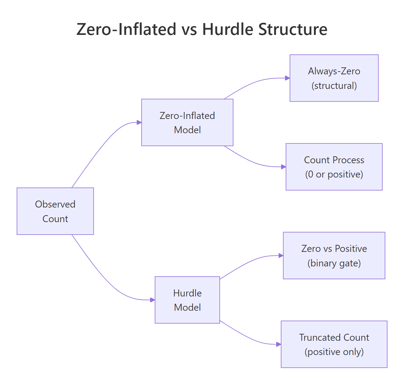
Figure 1: The two model families split the count process differently: zero-inflated mixes a structural-zero class with a count process, while hurdle uses a binary gate followed by a zero-truncated count.
The math makes the difference concrete. For a zero-inflated Poisson with parameters $\pi$ (structural-zero probability) and $\lambda$ (count rate):
$$ P(Y = y) = \begin{cases} \pi + (1 - \pi) \cdot e^{-\lambda} & \text{if } y = 0 \\ (1 - \pi) \cdot \dfrac{\lambda^y \, e^{-\lambda}}{y!} & \text{if } y > 0 \end{cases} $$
Where:
- $Y$ = the observed count (e.g., articles published)
- $\pi$ = probability of being a structural zero (a person who would never publish)
- $\lambda$ = Poisson rate for the regular count process
- $e^{-\lambda}$ = Poisson probability of a "sampling" zero, which adds to the structural zeros
The headline: a ZIP model lets you observe a zero from either source, while a hurdle says all zeros come from the same gate. If you don't care about the math, the diagram and the next two sections give you everything you need.
A quick visual check shows why these models exist for bioChemists:
About 275 students sit in the zero bar alone, and the bars decay rapidly from 1 to 7. Any single-distribution fit has to make a brutal trade-off: explain the zeros well or explain the tail well, but not both.
Try it: Compute the variance-to-mean ratio of bioChemists$art to confirm that overdispersion (variance > mean) is also present, which is what motivates negative-binomial variants of these models.
Click to reveal solution
Explanation: A ratio of 3.7 means the variance is nearly four times the mean, well above the Poisson assumption of equality. That is why ZINB and hurdle-NB usually beat their Poisson cousins on this dataset.
How do you fit a zero-inflated Poisson with pscl::zeroinfl()?
The zeroinfl() formula has two pipes: the part before | describes the count process, the part after describes the structural-zero process. Using . on both sides applies all predictors to both components, which is the right starting point when you don't have strong priors about which variables affect each part.
The output is two regressions stacked. The count component reads like a normal Poisson: women publish about $e^{-0.21} \approx 0.81$ as many articles as men, and each additional mentor publication multiplies the student's expected count by $e^{0.018} \approx 1.018$. The zero-inflation component is a logistic regression on whether the student is a structural zero (one who would never publish, regardless of effort): only ment is significant, and the negative coefficient means more-published mentors reduce the odds of having a structural-zero student.
How well does the ZIP close the 9-point gap from before?
The ZIP nails it: the average predicted P(Y=0) is 0.299, almost exactly the observed 0.300, and the Poisson's nine-point miss is gone. This is the easiest sanity check that the inflation component is doing real work.
Try it: Refit as a zero-inflated negative binomial by passing dist = "negbin". Compare the new theta (dispersion) parameter and the AIC.
Click to reveal solution
Explanation: The negative binomial absorbs overdispersion explicitly through theta, dropping the AIC by 16, strong evidence that ZINB is preferred over ZIP for this data.
How do you fit a hurdle model with pscl::hurdle()?
The hurdle() formula uses the same two-pipe syntax, but the components mean different things. Before | is now a zero-truncated count distribution that fires only when the gate is open. After | is a binary gate predicting whether art > 0 at all.
The count coefficients are nearly identical to ZIP because they are estimating the same quantity (the Poisson rate among publishers). What changes is the zero component: it is now a plain logistic regression on art > 0. Its coefficients are easy to interpret: a positive marMarried coefficient means married students are more likely to publish at least once, and kid5's negative sign says small children at home reduce that probability. No gymnastics with "structural" vs "sampling" zeros.
glm(art > 0 ~ ., family = binomial). That makes it easier to debug and to teach: you can fit the gate alone, sanity-check it, then layer the truncated count on top. ZIP cannot be decomposed this way because both components produce zeros.The hurdle says a married woman PhD with one young child, mid-tier program, and a productive mentor has a 77% chance of publishing at least once. Multiplying by the truncated count gives the full prediction.
Try it: Refit hurdle with dist = "negbin" and report which AIC is lower (Poisson hurdle vs NB hurdle).
Click to reveal solution
Explanation: The NB version of hurdle handles the long tail of high-publishing students much better, dropping the AIC by 12. The truncated negative binomial is the right tail distribution here.
How do you choose between ZIP, ZINB, and hurdle models?
Three knobs decide it: dispersion in the positive counts, whether your zeros are theoretically a separate population, and the data's verdict via AIC and the Vuong test. The diagram below sketches the practical decision tree.
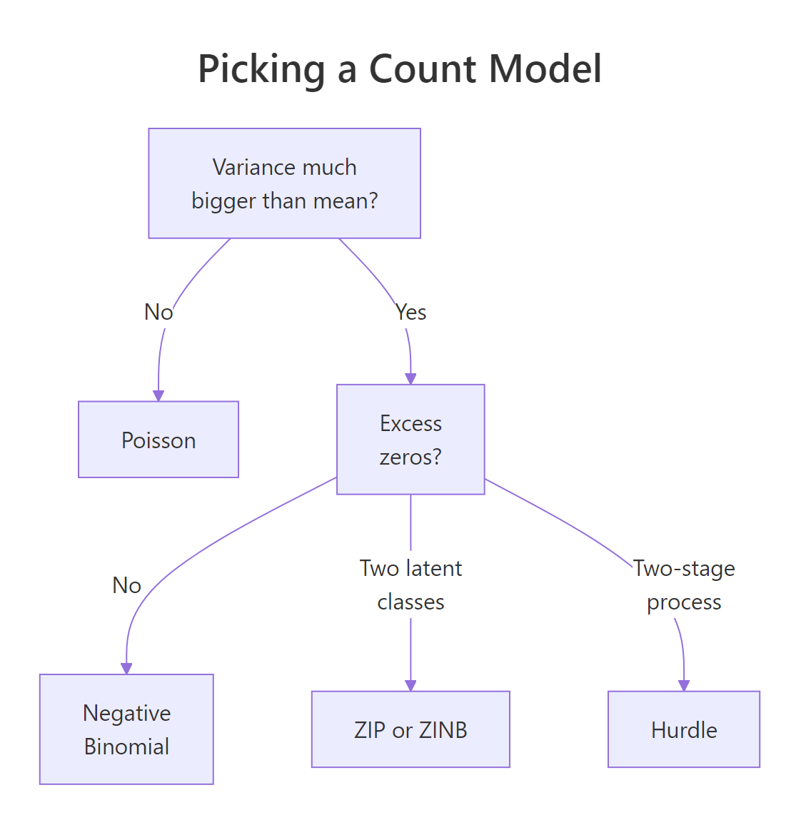
Figure 2: Decision flow for picking between Poisson, negative binomial, zero-inflated, and hurdle models based on dispersion and zero-rate diagnostics.
A head-to-head AIC ranking is the fastest data-driven check. Lower AIC is better and a difference of 2 or more is conventionally meaningful.
Hurdle-NB edges out ZINB by about 3 AIC points, and both leave plain Poisson 100 points behind. Whenever ZINB and hurdle-NB are within a few AIC points, the practical choice should fall back to interpretation: do you have a story about structural zeros, or about a gate?
The Vuong test gives a formal head-to-head between non-nested models, comparing the model-implied likelihood for each observation:
model2 > model1 with z-statistic of about -6.9 means ZIP is overwhelmingly better than vanilla Poisson, every correction agrees and the p-value is effectively zero. Vuong is most useful when AIC differences are small or when you want a hypothesis-test framing rather than information criteria.
Try it: Rank all six models by AIC and identify the winner programmatically.
Click to reveal solution
Explanation: order() returns row indices sorted by the AIC column. Hurdle-NB tops the table, then ZINB, then Poisson hurdle, all NB-flavoured variants beat their Poisson cousins because of overdispersion in the positive-count tail.
Practice Exercises
Exercise 1: AIC delta between ZINB and hurdle-NB
Compute the AIC of m_zinb and m_hurdle_nb, take their difference, and decide which model is preferred (a positive difference favours m_hurdle_nb because it has the lower AIC).
Click to reveal solution
Explanation: A positive delta means ZINB has a higher AIC, so the hurdle-NB is preferred by a small but meaningful margin.
Exercise 2: Decompose ZIP's predicted zeros
For each row, the ZIP-predicted P(Y=0) has two parts: a structural part ($\pi$) from the zero component, and a Poisson-zero part ($(1-\pi) e^{-\lambda}$) from the count component. Compute the average of each part separately and verify they add to the total predicted zero rate.
Click to reveal solution
Explanation: ZIP attributes about 9 of every 30 zero observations to the structural class, and the remaining 21 to ordinary Poisson sampling at low $\lambda$. The two pieces sum to the model's predicted zero rate.
Exercise 3: Compare ZIP and hurdle predictions for one profile
Predict the expected article count for a hypothetical female biochemist with mar = "Married", kid5 = 2, phd = 3.5, ment = 8 under both m_zip and m_hurdle, and explain why they differ.
Click to reveal solution
Explanation: Both models predict around one article for this profile, but the hurdle's truncated Poisson conditions on art > 0, so its expected positive count is slightly higher than the ZIP's mixture of "always-zero" plus "Poisson with the same rate". The two stories give similar headline numbers but different mechanism narratives.
Complete Example
The end-to-end workflow on bioChemists is a good template you can drop onto any count outcome.
Hurdle-NB wins by a hair on AIC, and Vuong does not strongly favour either it or ZINB. Because the substantive question reads naturally as "did the student publish at all → if so, how many?", we keep the hurdle. The count component says women publish about $e^{-0.24} \approx 0.78$ times as many articles as men among publishers, and the binary gate says the same effect (women are slightly less likely to cross the hurdle, $e^{-0.25} \approx 0.78$).
Summary
| Model | Use when... | pscl call | |
|---|---|---|---|
| Poisson | Mean ≈ variance, observed zero rate matches dpois(0, fitted) |
glm(..., family = poisson) |
|
| Negative Binomial | Variance > mean, no excess zeros after accounting for dispersion | MASS::glm.nb() |
|
| ZIP / ZINB | Excess zeros and you can story-tell two latent classes | `zeroinfl(... \ | ...)` |
| Hurdle / Hurdle-NB | Excess zeros and a clean two-stage process | `hurdle(... \ | ...)` |
Three rules of thumb cover most cases. First, always run the observed-vs-predicted zero-share diagnostic before reaching for ZIP or hurdle, if Poisson already nails the zero rate, you are wasting parameters. Second, prefer the negative-binomial flavour (dist = "negbin") whenever the variance-to-mean ratio is much greater than 1, which is most of the time. Third, when AIC and Vuong leave you indifferent between ZIP and hurdle, let the substantive interpretation break the tie: structural zeros vs two-stage gate is rarely an empirical question.
References
- Zeileis, A., Kleiber, C. & Jackman, S., Regression Models for Count Data in R. Journal of Statistical Software (2008). Vignette PDF
- pscl package, CRAN. Link
- Cameron, A. C. & Trivedi, P. K., Regression Analysis of Count Data, 2nd edition. Cambridge University Press (2013).
- UCLA OARC, Zero-Inflated and Hurdle Models for Count Data in R. Link
- Vuong, Q. H., Likelihood ratio tests for model selection and non-nested hypotheses. Econometrica (1989). JSTOR
- Mullahy, J., Specification and testing of some modified count data models. Journal of Econometrics (1986).
- Long, J. S., Regression Models for Categorical and Limited Dependent Variables. Sage (1997). Source of the
bioChemistsdataset.
Continue Learning
- Poisson & Negative Binomial Regression: Model Count Data in R, the prerequisite parent post that fits and interprets the simpler count models on
quineand other examples. - Logistic Regression in R, the binary classifier behind every hurdle model's gate component.
- Generalized Linear Models in R, the unifying GLM framework that all five models in this post extend.