R Data Frames: Every Operation You'll Need, With 10 Real Examples
A data frame in R is a table of rows and columns, like a spreadsheet or a database table, where each column can be a different type. It's the single most important data structure for real analysis work, and it powers everything from lm() to ggplot2.
What is an R data frame and how do you build one?
Under the hood, a data frame is just a list of equal-length vectors, with each vector being one column. That's why columns can be different types (numeric, character, logical) but a column itself must be one type. Let's build one and look at it.
Five rows, four columns, two types (numeric and logical plus character). That's a typical data frame in a realistic shape. You'll build many of these from scratch for demos, tests, and quick prototypes, and many more from read.csv() when you load real data.
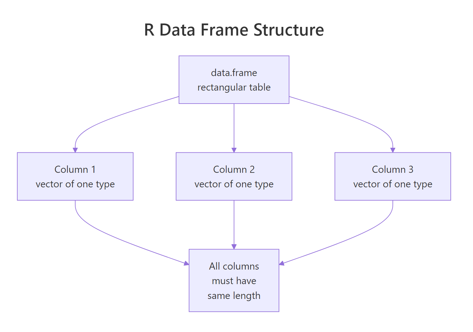
Figure 1: A data frame is a list of equal-length column vectors. Each column has a type; each row spans all columns.
stringsAsFactors = TRUE by default, which silently turned character columns into factors. That default is gone, but you'll still see tutorials setting stringsAsFactors = FALSE explicitly, harmless, but no longer required.Try it: Build a data frame with three cities, their populations, and whether they're coastal.
Click to reveal solution
Each argument to data.frame() becomes one column, and the three input vectors all have length 3 so the rows line up automatically. Because each column can hold a different type, character, numeric, logical, you get a small mixed-type table in one call.
How do you inspect a data frame?
Before you touch a new data frame, you want a quick profile: how big is it, what types are the columns, what's in the first few rows? R gives you a handful of inspection functions that together answer every "what am I looking at?" question.
str() is the workhorse, it tells you shape, column names, types, and a preview in one line per column. summary() gives five-number summaries for numeric columns and counts for factors/characters.
Try it: Print the names of all columns in employees using names() or colnames().
Click to reveal solution
names() returns the column names of a data frame as a character vector, which is the same thing colnames() gives you. Prefer names() in base R because it's shorter and works on lists too.
How do you select columns?
There are four ways to pull a column out of a data frame, and you'll see all of them in real code. Let's work through them, because the differences matter, especially when one returns a vector and another returns a one-column data frame.
The first three return the column as a plain vector. The fourth, selecting multiple columns, returns a smaller data frame. That asymmetry is a classic R gotcha: df[, "x"] is a vector, but df[, c("x", "y")] is a data frame.
df$col for quick interactive work, df[["col"]] when the column name is in a variable, and df[, cols] (with a character vector) when you want a sub-data-frame with multiple columns.Try it: Pull just the age column out of employees as a vector, then compute its mean.
Click to reveal solution
employees$age returns the age column as a plain numeric vector, which is exactly what mean() expects. The mean of c(29, 42, 31, 55, 38) is 195/5 = 39.
How do you filter rows?
Filtering rows is the operation you'll do most often. In base R, you index with a logical vector in the row position: df[condition, ]. The comma is critical, it says "all columns." Leave it out and R gets confused.
Combine conditions with & (and) and | (or). Never use && or ||, those are scalar operators for single TRUE/FALSE values, not vectors.
df[df$x > 5] (without the comma) silently picks columns whose position matches the logical vector's TRUEs, not rows. Always include the comma: df[df$x > 5, ].Try it: Filter employees to rows where salary is below 75000.
Click to reveal solution
employees$salary < 75000 is a logical vector aligned with the rows, and using it in the row position of [ , ] keeps only the rows that match. Remember the trailing comma, it tells R "all columns" and is the difference between filtering rows and accidentally picking columns.
How do you add or modify columns?
Adding a column is the same syntax as selecting one, just assign into it. This works whether the column already exists (modify) or doesn't (create). The new column can be a constant, a vector, or a vectorized computation on existing columns.
ifelse() is the vectorized counterpart to the scalar if/else, it applies the condition element-by-element across the vector. To drop a column, assign NULL: employees$bonus <- NULL.
Try it: Add a column high_earner that is TRUE when salary is above 80000.
Click to reveal solution
Assigning into a new name, employees$high_earner, appends a column because the name doesn't exist yet. The right-hand side is a vectorized comparison, so R broadcasts > 80000 across every salary and stores the logical result as the new column.
How do you sort and rank rows?
Sorting a data frame means reordering its rows by one or more columns. Base R uses order(), which returns the positions that would put a vector in sorted order. You then use those positions as a row index.
A negative sign in front of a numeric column reverses that column's sort order. For character/factor columns, wrap them in order(..., decreasing = TRUE) instead.
Try it: Sort employees by age ascending.
Click to reveal solution
order(employees$age) returns the row positions that would sort age ascending, c(1, 3, 5, 2, 4), and indexing with them reorders the data frame. Notice the row numbers on the left: they carry over from the original, which is how you can tell sorting rearranged rows rather than rebuilding the data frame.
How do you summarize by group with aggregate()?
The "split-apply-combine" pattern, group rows by a column, compute something on each group, combine the results, is the core of most analyses. Base R's aggregate() does it in one call.
The ~ is formula syntax: "compute this on the left, grouped by that on the right." You can supply any function, sum, median, sd, or a custom one. For heavier aggregation work you'll eventually reach for dplyr::group_by() + summarise(), but aggregate() is perfect when you want zero dependencies.
aggregate() drops rows where the grouping column is NA. If you need to keep them, convert NA to a sentinel string first.Try it: Compute the maximum salary grouped by remote.
Click to reveal solution
The formula salary ~ remote says "compute on salary, split by remote", and passing max as FUN applies it to each group. David (non-remote) has the highest overall salary at 95000, while Eve tops the remote group at 78000.
Practice Exercises
Exercise 1: Top earners by department
Build a data frame of 8 employees across 3 departments, then return the top earner in each.
Show solution
Exercise 2: Filter and summarize
From mtcars, return the mean mpg for 4-cylinder cars weighing under 2.5.
Show solution
Exercise 3: Add a categorical column
Add a column mpg_class to mtcars: "low" if mpg < 18, "mid" if 18-25, "high" if > 25. Then count the rows in each class.
Show solution
Putting It All Together
A complete mini-analysis on iris, load it, inspect, filter, add a derived column, sort, and summarize by species.
Five operations, five lines, and every single one is a base-R idiom you'll reach for daily.
Summary
| Operation | Syntax |
|---|---|
| Create | data.frame(col1 = ..., col2 = ...) |
| Inspect | str(), dim(), head(), summary() |
| Select column | df$col, df[["col"]], df[, "col"] |
| Filter rows | df[df$col > 5, ], don't forget the comma |
| Add column | df$new <- ... |
| Drop column | df$col <- NULL |
| Sort | df[order(df$col), ] |
| Group summary | aggregate(y ~ g, data = df, FUN = mean) |
References
- R Language Definition, Data Frames
- Advanced R, Data Frames by Hadley Wickham
- R for Data Science, modern tidyverse perspective on tables
- Base R Cheat Sheet (RStudio)
- An Introduction to R, Chapter 6: Lists and data frames
Continue Learning
- R Lists: When Data Frames Aren't Flexible Enough, the more flexible cousin of data frames.
- R Vectors: The Foundation of Everything in R, understand the columns that data frames are built from.
- R Data Types: Which Type Is Your Variable?, know the types each column can hold.
Further Reading
- Why R Copies Your Data (And How Copy-on-Modify Actually Saves Memory)
- R Matrices: Fast Linear Algebra Operations That Data Frames Can't Do
- Data Frame Exercises in R: 17 Real-World Practice Problems
- tibble add_column() in R: Append Columns to a Data Frame
- tibble add_row() in R: Append Rows to a Data Frame
- tibble as_tibble() in R: Convert Objects to Tibbles
- tibble as_tibble_col() in R: Vector to One-Column Tibble
- tibble as_tibble_row() in R: One Row at a Time
- tibble column_to_rownames() in R: Move Column Into Rownames
- tibble rownames_to_column() in R: Move Rownames to Column
- tibble tibble() in R: Build Tibbles Column by Column
- tibble tribble() in R: Build Tibbles Row by Row
- tibble deframe() in R: Two-Column Tibble to Named Vector
- tibble enframe() in R: Named Vector to Two-Column Tibble
- tibble glimpse() in R: Compact Transposed Data Preview
- tibble has_rownames() in R: Detect Non-Trivial Row Names
- tibble remove_rownames() in R: Strip Row Names Cleanly
- tibble rowid_to_column() in R: Add Sequential Row IDs