Bivariate EDA in R: Find Relationships Between Variables Before You Model Them

Bivariate EDA examines how two variables move together — through scatter plots, grouped boxplots, bar charts, and correlation measures — so you can spot relationships, confounders, and surprises before building any model.

How Do You Explore Two Numeric Variables?

Before you model anything, you need to know which variables are actually related. Bivariate EDA answers that question with the right plot paired with the right summary statistic — and the choice depends on whether each variable is numeric or categorical. Let's start with the most common scenario: two numeric variables and a scatter plot that reveals their relationship instantly.

The downward-sloping line tells you immediately: bigger engines burn more fuel on the highway. The grey confidence band is narrow in the middle (where most data sits) and wider at the extremes — that's your uncertainty growing where data is sparse.

Now let's put a number on that relationship. A correlation coefficient ranges from -1 (perfect negative) to +1 (perfect positive), with 0 meaning no linear relationship.

Both Pearson and Spearman confirm a strong negative correlation. Spearman's rho is slightly stronger here (-0.833 vs -0.766) because it captures the monotonic relationship even if the curve isn't perfectly straight. The p-values are astronomically small — this relationship is not a coincidence.

Sometimes a third variable hides inside a bivariate relationship. Colouring by drv (drive type) reveals subgroup trends that the overall scatter plot blurs together.

Now you can see that front-wheel drive cars dominate the small-engine, high-mpg corner, while rear-wheel drive cars cluster among large engines. The overall trend isn't wrong — but it's masking three distinct stories.

What If One Variable Is Categorical and the Other Numeric?

When one variable is a group label — like vehicle class, species, or treatment arm — and the other is a measurement, you want to see how distributions shift across groups. The grouped boxplot is the workhorse here: it shows median, spread, and outliers in one compact visual.

Ordering the categories by median (using fct_reorder()) makes the comparison instant — you don't have to scan alphabetically. Pickups and SUVs cluster low; compact and midsize cars sit high. The red dots are outliers — individual cars that deviate from their class's pattern.

Violin plots reveal the density shape that boxplots hide. Overlaying jitter points shows each individual observation — especially valuable for small samples where the density estimate gets noisy.

The violin shape confirms that all three species have roughly unimodal distributions, but virginica has the widest spread. The jitter dots let you see that setosa's 50 observations cluster tightly — the violin isn't misleading.

Sometimes you want a cleaner summary: just the group means with error bars. The stat_summary() function handles this without any manual data wrangling.

Error bars that don't overlap suggest the group means are meaningfully different. The compact class clearly separates from SUVs and pickups — but midsize and compact overlap, so you'd need a formal test to distinguish them.

How Do You Compare Two Categorical Variables?

When both variables are categories — like vehicle class and drive type, or treatment and outcome — you need to see how frequencies cluster across combinations. A grouped bar chart shows raw counts; a proportional stacked bar reveals compositional differences.

The pattern is striking: SUVs are overwhelmingly 4-wheel drive, compacts are almost entirely front-wheel, and 2-seaters are all rear-wheel. That's a strong association between class and drive type — not independent at all.

Let's test that association formally with a contingency table and chi-squared test. The chi-squared test asks: "Could this frequency pattern have appeared by chance if class and drive type were truly independent?"

A chi-squared statistic of 291.6 with 12 degrees of freedom and a p-value near zero means these variables are very strongly associated. Vehicle class and drive type are far from independent.

A proportional stacked bar chart normalizes each class to 100%, making it easy to compare compositions even when group sizes differ.

Now the compositional story is crystal clear: pickups are exclusively 4-wheel, minivans are exclusively front-wheel, and SUVs are overwhelmingly 4-wheel with a rear-wheel minority. This proportional view is far more informative than raw counts when group sizes vary.

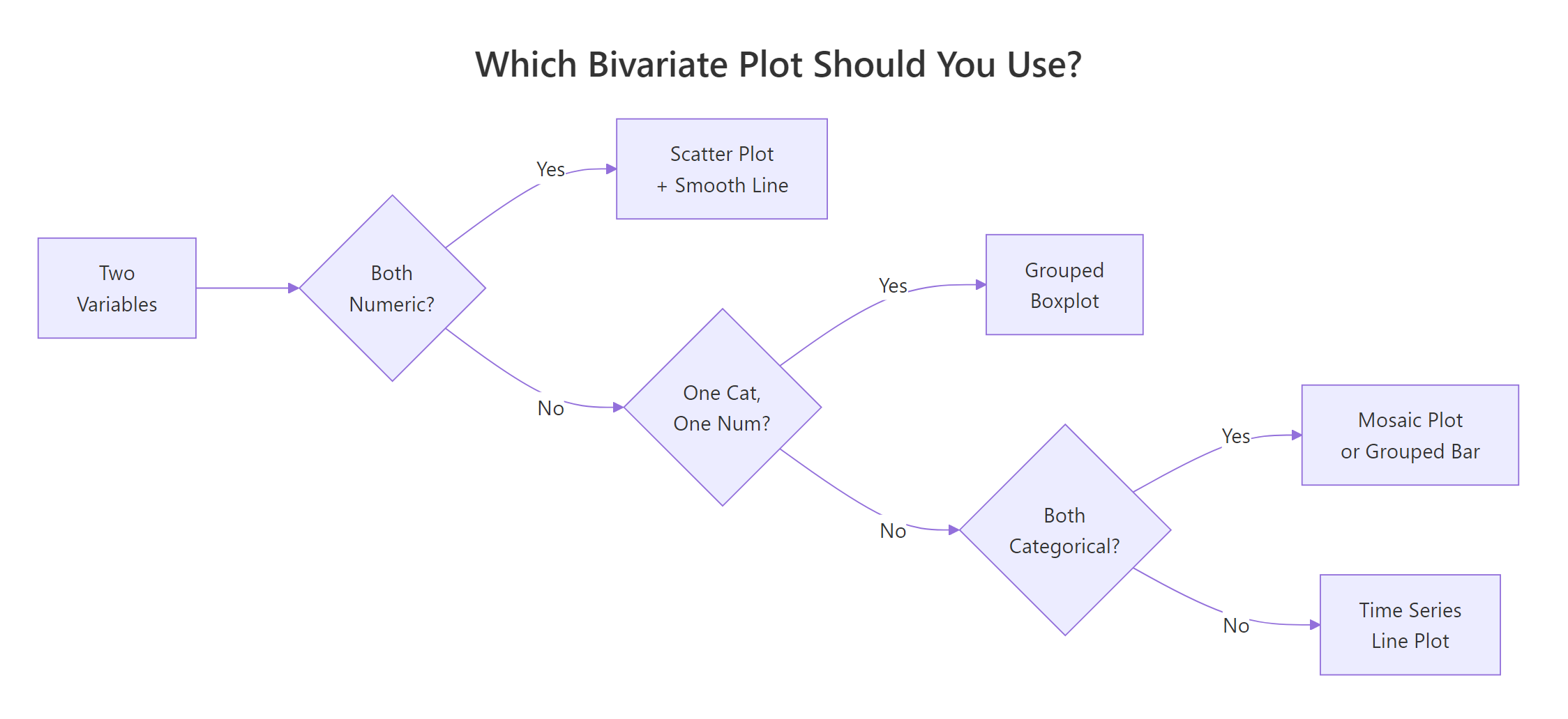
Which Plot Should You Pick for Each Variable Pair?

The single most important decision in bivariate EDA is matching the plot to the variable types. Here's the decision table to bookmark.

Figure 1: Which bivariate plot to use, based on variable types.

Let's see all three plot types side by side on the same dataset. The patchwork package makes this effortless.

Seeing all three together reinforces the core lesson: the variable types dictate the plot, and the plot dictates which summary statistic to compute. Pick the wrong plot and you'll miss the pattern entirely.

How Do You Scan All Pairs at Once with ggpairs()?

When you have four or more variables, checking every pair one-by-one gets tedious fast. GGally's ggpairs() builds a scatterplot matrix that automatically picks the right chart for each variable combination: scatter plots for numeric × numeric, boxplots for categorical × numeric, and bar charts for categorical × categorical.

Reading this matrix is straightforward: the diagonal shows each variable's distribution, the upper triangle gives you the correlation numbers, and the lower triangle shows the actual scatter plots. Colour-coding by drv reveals that front-wheel drive cars cluster in the low-displacement, high-mpg corner.

You can customize every panel. The upper triangle can show correlation coefficients, the lower can show scatter plots with smooth lines, and the diagonal can show densities or histograms.

The iris matrix instantly reveals that petal dimensions (length and width) are almost perfectly correlated (r = 0.96) and provide strong species separation. Sepal width is the odd one out — weakly correlated with everything and overlapping across species.

What Traps Should You Watch for in Bivariate EDA?

Bivariate EDA can mislead if you don't watch for common pitfalls. The three biggest traps are Simpson's paradox, nonlinear relationships that correlation misses, and overplotting that hides density patterns.

Simpson's paradox is when an aggregate trend reverses once you split by a third variable. Let's simulate this to see it happen.

The dashed black line slopes downward — suggesting a negative relationship. But both group-level lines slope upward. The paradox happens because Group B has higher x-values but lower y-values than Group A, creating a downward illusion when you ignore the group.

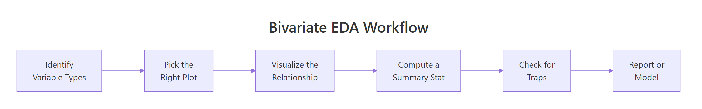
Figure 2: The bivariate EDA workflow from variable identification to reporting.

Nonlinear relationships are the second trap. A correlation coefficient measures linear strength, so a perfect curve can produce r ≈ 0.

The scatter plot shows an obvious quadratic pattern, but Pearson's r is essentially zero. This is exactly why "always plot first" is the golden rule. Spearman wouldn't help here either — the relationship isn't monotonic.

Overplotting is the third trap. When thousands of points stack on top of each other, you can't see where the data actually concentrates. Here's how to fix it with transparency and 2D binning.

The alpha-transparency version shows faint structure — bands at 0.5, 1.0, and 1.5 carats where diamonds are cut to round numbers. The 2D bin version makes this density pattern unmistakable with a color scale. For any dataset with more than a few thousand points, one of these two approaches (or hexbin, covered next) is essential.

How Do You Handle Large Datasets with Many Variables?

With thousands of rows or dozens of columns, individual scatter plots become unreadable and pair matrices become impractical. A correlation heatmap gives you a bird's-eye view of which numeric pairs are worth investigating, and hexbin plots handle the overplotting problem for large scatter plots.

The heatmap instantly highlights the strongest relationships. The darkest red cells (disp-cyl, wt-disp) and darkest blue cells (mpg-wt, mpg-cyl) are the pairs worth exploring further with scatter plots. The near-white cells are pairs you can skip.

For large datasets like diamonds (53,000+ rows), hexbin plots are the best alternative to point scatter plots. Each hexagon represents a bin and is colored by the count of observations it contains.

The hexbin plot reveals that the relationship between carat and price is nonlinear — price accelerates as carat increases. Most diamonds cluster in the small-carat, low-price corner. A log-scale on the color fill helps distinguish density differences in the sparse upper region.

Practice Exercises

Exercise 1: Does Better Cut Mean Higher Price?

Using the diamonds dataset, create a grouped boxplot of price by cut, then compute the mean price per cut level. Does the "best" cut (Ideal) have the highest price? Explain why or why not.

Exercise 2: Complete Bivariate EDA on mpg

Build a complete bivariate EDA of the mpg dataset. Create three plots: (1) a scatter plot for displ vs cty, (2) a grouped boxplot for class vs cty, and (3) a proportional stacked bar for class vs fl (fuel type). Combine all three using patchwork.

Exercise 3: Demonstrate Simpson's Paradox with UCBAdmissions

The UCBAdmissions dataset contains admission decisions at UC Berkeley by gender and department. Show that overall admission rates appear to favour males, but within individual departments the pattern changes. Use appropriate plots.

Putting It All Together

Let's run a complete bivariate EDA on the mpg dataset, covering all four variable-pair types in one end-to-end workflow.

This six-step workflow — identify types, scatter, boxplot, bar/chi-squared, ggpairs, and summarize — gives you a complete picture of any dataset's bivariate relationships in minutes.

Summary

Here's a quick-reference table for every bivariate scenario you'll encounter.

Three rules to live by:

1. Always plot first, then compute. A correlation number without a scatter plot is dangerous — it can't detect nonlinear patterns or outlier influence.
2. Match the plot to the variable types. The decision table above is your starting point for every analysis.
3. Facet by a third variable before trusting an aggregate trend. Simpson's paradox is real and common.

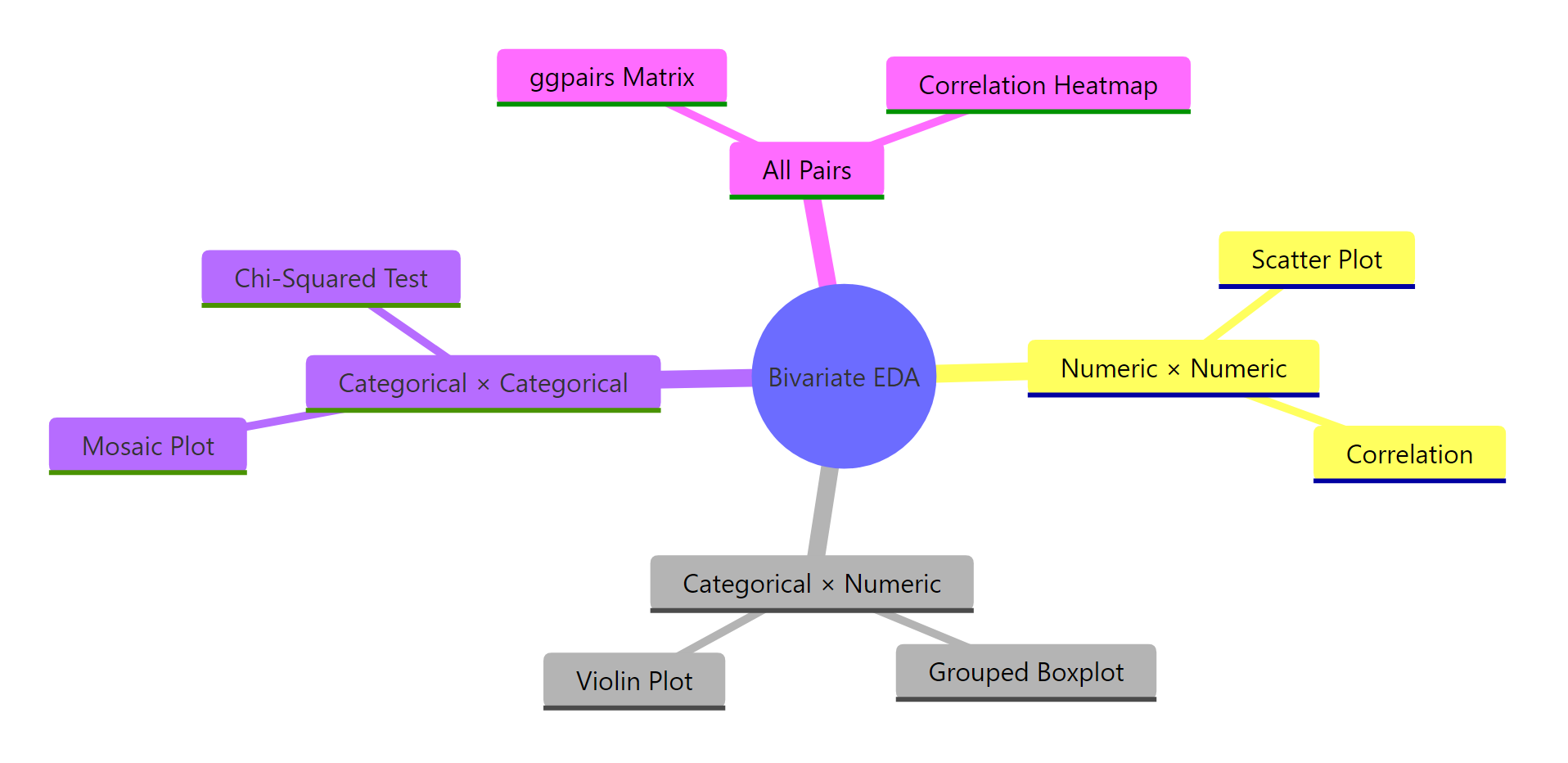
Figure 3: The main concepts and techniques in bivariate EDA.

References

1. Wickham, H. & Grolemund, G. — R for Data Science, 2nd Edition. O'Reilly (2023). Chapter 10: Exploratory Data Analysis. Link
2. Kabacoff, R. — Modern Data Visualization with R. Chapter 5: Bivariate Graphs. Link
3. ggplot2 documentation — geom_point() reference. Link
4. ggplot2 documentation — geom_boxplot() reference. Link
5. GGally documentation — ggpairs() reference. Link
6. R Core Team — cor.test(): Test for association/correlation between paired samples. Link
7. Tukey, J.W. — Exploratory Data Analysis. Addison-Wesley (1977).
8. Cleveland, W.S. — Visualizing Data. Hobart Press (1993).

Continue Learning

• Univariate EDA in R — Understand single-variable distributions before comparing pairs.
• Exploratory Data Analysis in R (7-Step Framework) — The complete EDA workflow from data import to actionable insight.
• Correlation Matrix Plot in R — Deep dive into multi-variable correlation visualization and interpretation.