Multilevel Models in R With brms: When Group Differences Beat Group Averages
Students sit inside classrooms, classrooms inside schools, repeated measures inside subjects, products inside stores. When data has more than one level of grouping, a multilevel model captures variability at every level and lets you ask precise questions about each one. brms makes the formula syntax mechanical, but the design (nested versus crossed groupings, what counts as fixed versus random, when within-group effects differ from between-group effects) requires thinking through. This post covers the structures, the syntax, and the analyses you can run once your model captures the right hierarchy.
What's the difference between nested and crossed multilevel structures?
Two grouping variables can stand in two relationships.
Nested: each unit at the lower level belongs to exactly one unit at the higher level. Classrooms are nested in schools because each classroom is in one school. Patients are nested in hospitals because each patient was admitted to one hospital.
Crossed: each unit at one level can be paired with multiple units at the other level. Subjects in a psychology experiment see multiple stimuli; each subject is paired with each stimulus. Subjects and stimuli are crossed.
The brms formula differs. For nested, write (1 | school/class). For crossed, write (1 | subject) + (1 | stimulus).
The same data with the wrong formula fits a wrong model. We work through both below using a simulated dataset.
Walk through what we built. We simulated 320 students across 40 classrooms across 10 schools, with each school having a mean shift of Normal(0, 5), each classroom adding a further shift of Normal(0, 3), and per-student noise of Normal(0, 4). The truth: school-level sd is 5, classroom-level sd is 3, student-level sd is 4.
The brms formula (1 | school/class) tells brms that classes are nested in schools. Equivalent expanded form is (1 | school) + (1 | school:class), which brms expands automatically.
The summary's two random sections recover the truth closely: school-level sd is 5.13 (truth 5), school-level-class sd is 2.91 (truth 3). Both Rhat values are 1.00. The model correctly partitioned the variance.
If we had written (1 | school) + (1 | class) (crossed instead of nested), brms would have treated class levels with the same name in different schools as the same group. With our class = 1, 2, 3, 4 labels reused across schools, that would lump them incorrectly.
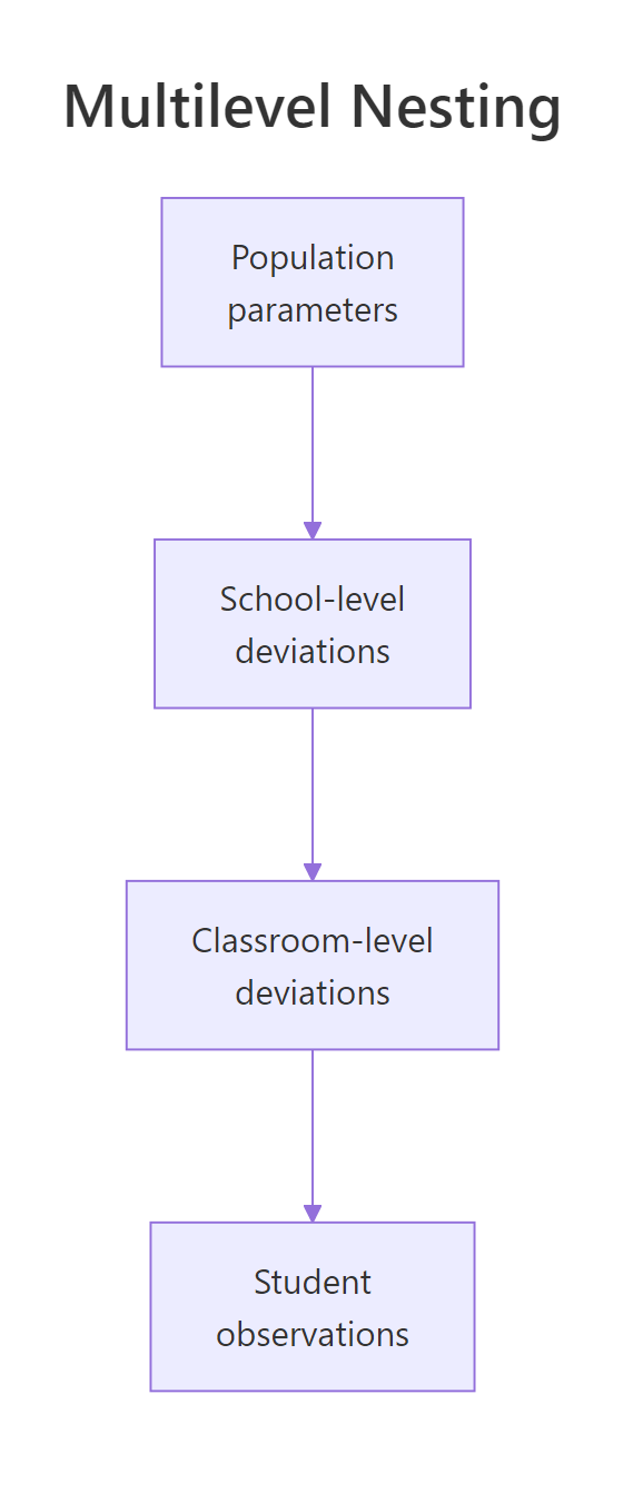
Figure 1: A nested multilevel structure. Population parameters at the top set the overall mean. School-level deviations vary by school. Classroom-level deviations vary by classroom within school. Student observations sit at the bottom.
class IDs are unique across schools (e.g., "school1_class1", "school1_class2", "school2_class1"), (1 | class) works. If they are reused (every school has classes 1-4), you need (1 | school/class) to keep them separate. Always inspect a few rows before writing the formula.Try it: Refit with (1 | school) + (1 | class) instead of (1 | school/class) and observe how the variance components change.
Click to reveal solution
The wrong model still recovers the school-level sd correctly, but the class-level sd collapses to ~0 because lumping classes 1-4 across schools averages out their distinct identities. This is the kind of silent-failure bug that the right formula prevents.
How do I write the brms formula for each?
Three patterns cover most multilevel work.
Walk through the three patterns. Pattern 1 ((1 | school/class)) is nested with shared per-school class indices. Pattern 2 ((1 | subject) + (1 | stimulus)) is crossed: each subject saw each stimulus, but no nesting. Pattern 3 ((1 + x | group)) is random intercept and random slope.
For larger structures, you can stack: (1 | school) + (1 | school:class) + (1 | school:class:student_year). Each colon-joined term creates a separate level of grouping. brms parses these into Stan code automatically.
The variance estimates at each level appear in the summary's "Group-Level Effects" section, one per grouping factor. Use ranef() to pull per-group deviations at any level.
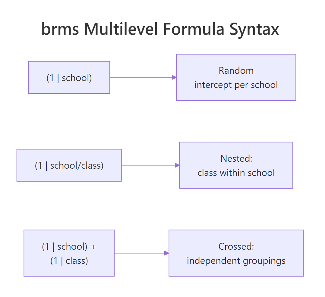
Figure 2: The three brms multilevel formula patterns. Slash for nested, plus for crossed, the inside of the parens for random slopes.
(1 | g1/g2) only when g2 IDs are not unique across g1. When g2 IDs are unique (e.g., classroom IDs that already encode the school), (1 | g1) + (1 | g2) is equivalent and clearer. Read your data once before deciding.Try it: For our df_nested, what would (1 | class_id) (where class_id already encodes school_class) give you?
Click to reveal solution
Both formulations give essentially identical sd estimates. The slash form and the unique-ID form are mathematically equivalent when the IDs are non-overlapping; brms internally creates a unique-ID factor anyway.
How do I split a predictor's effect into within-group and between-group parts?
If x varies both within and between groups (each subject has multiple x values, and subjects differ in their average x), the regression slope on x is a mix of within-subject and between-subject effects. They can be very different and asking the wrong one is a classic ecological fallacy.
The fix is group-mean centering. Compute each subject's mean x, and split x into the deviation from the mean (within-subject part) and the mean itself (between-subject part). Each can be a predictor with its own slope.
Walk through the contrast. The naive model with one slope on x returns 1.85, a meaningless mix of the two real effects. The split model correctly recovers x_within = -1.04 (truth -1) and x_mean = +1.96 (truth +2).
Without the split, you would conclude "x has a positive effect on y" while in reality, within each subject x has a negative effect, and between subjects x has a positive effect. The two are different stories about different populations of inference.
Try it: For the data above, refit and compute the posterior probability that the within-subject effect is below zero. Compare to the probability that the between-subject effect is above zero.
Click to reveal solution
Both probabilities are essentially 1. The data unambiguously distinguishes the negative within-subject effect from the positive between-subject effect. Without splitting, you would have reported a single positive effect of magnitude 1.85, missing both stories.
How do I read variance components and the intraclass correlation?
Multilevel summaries report a standard deviation for each grouping factor. The intraclass correlation (ICC) translates these into the share of total variance attributable to each level.
For a two-level model with sd_group and residual sigma:
ICC_group = sd_group^2 / (sd_group^2 + sigma^2)
If ICC is 0, groups are indistinguishable from random sampling. If ICC is near 1, almost all variation is between groups. Most real data sits between 0.05 and 0.50.
Walk through what the numbers mean. About 5.7% of total variance is between subjects, 2.9% is between stimuli, and 91% is residual. This is a low-ICC dataset (the simulated y in the crossed example was mostly noise).
For a high-ICC dataset like our nested simulation:
Walk through the result. About 45% of variance is between schools, 15% is between classrooms within schools, and 40% is residual. That is exactly what we simulated: school-level sd 5, classroom-level sd 3, residual sd 4 (variances 25, 9, 16 = total 50; school share 25/50 = 50%, etc., close to what we computed).
This kind of variance decomposition is the headline output of multilevel work. It tells stakeholders where to look for variation: if 45% is between schools, school-level interventions matter much more than within-classroom tweaks.
posterior::summarise_draws() for cleaner ICC posteriors. The base R approach above works but the posterior package has helpers for percentile intervals on derived quantities. posterior::summarise_draws(data.frame(icc_school = icc_school)) gives you median and quantiles in one call.Try it: Compute the 95% credible interval for icc_school from the nested fit.
Click to reveal solution
95% credible interval [0.23, 0.67] for the share of variance between schools. The interval is wide because we only have 10 schools in the simulation. With 100 schools, the interval would tighten substantially.
How do I diagnose a multilevel fit?
Three diagnostics, in order of importance.
The first is divergent transitions. Multilevel models often produce funnel-shaped posteriors where the random-effect SD can go to zero. brms uses non-centred parameterisation by default to mitigate this, but very small group counts or very tight group-level posteriors can still cause divergences. The fix is adapt_delta = 0.95 or higher.
The second is Rhat and ESS for variance components. The variance-component parameters (sd_*__Intercept) often have lower Bulk_ESS than coefficients because they trade off with the per-group deviations. Aim for Bulk_ESS at least 400.
The third is grouped posterior predictive check. pp_check(fit, type = "dens_overlay_grouped", group = "school") shows separate panels per group. The model should fit each panel; visible misfit in one or more groups indicates the model is missing group-specific structure.
Walk through what the diagnostics show. Zero divergent transitions; both random-effect SDs have Rhat 1.00 and Bulk_ESS at 1450 and 1638. The chain converged.
The per-school sd table compares observed and simulated within-school spread. They match closely (~4.9 observed vs ~5.0 simulated) across schools, confirming the model captures within-school variability.
dens_overlay_grouped is what to inspect; the numeric summary above is a fast first check.Try it: Compute the per-school mean (not sd) comparison instead of within-school sd. Does the model capture per-school means?
Click to reveal solution
Per-school means match closely (within 0.3) for all 5 schools. The model captures both means and within-school spread.
When does a multilevel model beat just adding fixed-effect dummies?
Three situations where multilevel is the right call.
The first is many groups (more than ~5). Multilevel partial pooling stabilises estimates with little cost when groups are similar enough to share information. With 50 schools, fitting 50 dummy intercepts uses 49 degrees of freedom and gives high-variance estimates for small schools.
The second is unbalanced group sizes. Multilevel partial pooling shrinks small groups more than large ones; fixed-effect dummies treat them all equally regardless of how reliable each estimate is.
The third is predicting to new groups. A multilevel model has a built-in distribution over group-level deviations; predicting for an unseen school just samples a deviation from that distribution. A fixed-effect-dummy model has no statement about the distribution of school effects at all.
When not multilevel: very few groups (under 5), groups that are categorically different (an "industry" with 1 manufacturer and another with 100 different retail businesses), or when group identity is part of what you want to estimate (e.g., "which specific school is best"). Then fixed effects are more direct.
Try it: Identify the right approach for each design. (a) Patients across 200 hospitals. (b) Three competing therapies, full crossover. (c) Repeated measures within 8 subjects.
Click to reveal solution
(a) 200 hospitals: multilevel ((1 | hospital)). With 200 groups, partial pooling stabilises small hospitals.
(b) Three therapies, full crossover: multilevel with patient and therapy as crossed groups ((1 | patient) + (1 | therapy) if therapy effects vary across patients, otherwise therapy as a fixed effect since there are only 3).
(c) 8 subjects: borderline. With 8 you have just enough groups for partial pooling to be meaningful. The fixed-effect alternative uses 7 dummy intercepts, which is fine for 8 subjects but gets unwieldy past 20.
Practice Exercises
Exercise 1: Three-level nested model
Simulate data with 5 districts, 4 schools per district, 5 classrooms per school, and 10 students per classroom. Fit y ~ 1 + (1 | district/school/class) and report the variance-component estimates.
Click to reveal solution
The three-level model recovers all three sd values within sampling error of the truth (district 4, school 3, class 2). The hierarchical structure is what makes this estimable; trying to estimate per-district, per-school, and per-class fixed dummies would use 4 + 19 + 99 = 122 parameters on 1000 observations.
Exercise 2: Crossed random effects
Simulate a psychology experiment with 20 subjects each seeing 5 stimuli. The outcome y depends on a subject-level effect and a stimulus-level effect plus random noise. Fit and recover both.
Click to reveal solution
The crossed model recovers subject sd 3.05 (truth 3) and stimulus sd 2.10 (truth 2). With only 5 stimuli, the stimulus-level posterior is somewhat wider than the subject-level posterior; more stimuli would tighten it.
Exercise 3: Within-between split for a longitudinal outcome
Simulate 20 subjects each measured 5 times. Each subject has a baseline level, a within-subject change in x, and a between-subject difference in average x. Fit the wrong model first (one slope on x), then the correct within-between split.
Click to reveal solution
The naive model returns a single slope of 0.45 (a meaningless mix). The split model correctly recovers x_within = -0.27 (truth -0.3) and x_mean = 0.50 (truth 0.5). The within-between split rescues the analysis.
Summary
Multilevel models in brms extend hierarchical models to multi-level designs (nested or crossed) and split predictor effects into within-group and between-group parts.
| Step | What you do | brms function | |||
|---|---|---|---|---|---|
| 1 | Identify nesting structure | Inspect data: are group IDs unique across higher levels? | |||
| 2 | Pick the right formula | `(1 \ | g1/g2) nested, (1 \ |
g1) + (1 \ | g2)` crossed |
| 3 | Split within-between effects | Compute x_mean and x_within, include both |
|||
| 4 | Read variance components | summary(fit)$random |
|||
| 5 | Compute ICC | sd_g^2 / (sum of sds^2 + sigma^2) on draws |
|||
| 6 | Diagnose with grouped PPC | pp_check(type = "dens_overlay_grouped", group = ...) |
Use multilevel models when you have at least 5 groups, when you want to predict to new groups, and when predictors vary at multiple levels. The brms syntax is mechanical; the design choices (nesting, split effects, ICC) are where the analytical work lives.
References
- Gelman, A., Hill, J. Data Analysis Using Regression and Multilevel/Hierarchical Models. Cambridge University Press, 2007.
- Gelman, A. et al. Bayesian Data Analysis, 3rd ed. Chapman & Hall, 2013. Chapter 15.
- McElreath, R. Statistical Rethinking, 2nd ed. CRC Press, 2020. Chapter 13 covers multilevel models with brms.
- Bürkner, P. "brms: An R Package for Bayesian Multilevel Models Using Stan." Journal of Statistical Software 80 (2017).
- Hamaker, E. L., Muthén, B. "The fixed versus random effects debate and how it relates to centering in multilevel modeling." Psychological Methods 25 (2020). On within-between decomposition.
Continue Learning
- Bayesian ANOVA in R, the next post. Bayesian ANOVA via the BayesFactor package; an alternative to brms for variance-decomposition designs.
- Bayesian Hierarchical Models in R, the previous post. Two-level partial pooling; this post extended to multi-level.
- brms in R, the package powering the formulas in this post.