Expected Value and Variance: Derive Them Theoretically, Then Verify via Simulation
The expected value of a random variable is its long-run average, the probability-weighted mean of all outcomes. The variance measures how far typical outcomes sit from that average, squared. Derive each formula once, then verify it in seconds with a 10,000-draw R simulation. The sample statistic will close in on the theoretical value every time.
What is expected value, and why is it the long-run average?
A fair six-sided die lands on each face with probability 1/6. You will never roll a 3.5 on a single toss, yet 3.5 is the right answer for "what do you expect on average." The expected value resolves that paradox. Here it is in code, with one line for the theoretical formula and another for the proof by simulation.
The sample mean landed at 3.50102, indistinguishable from the theoretical 3.5 at three decimal places. The formula sum(x * P(x)) is the entire definition of expected value for a discrete variable. Each face contributes its own value weighted by how likely it is, and you add them up. Simulation is just doing the weighting empirically instead of by formula.
For a general discrete random variable $X$ with outcomes $x_1, x_2, \ldots$ and probabilities $P(X = x_i)$:
$$E[X] = \sum_{i} x_i \cdot P(X = x_i)$$
The R pattern sum(vals * probs) computes this directly. You can also write it with weighted.mean(vals, probs) or c(vals %*% probs). All three return the same number.
Try it: A biased coin lands heads with probability 0.7. Define $X = 1$ when heads and $X = 0$ when tails. Compute $E[X]$ by formula, then verify with a simulation of 50,000 flips.
Click to reveal solution
Explanation: For a Bernoulli variable, $E[X] = p$ because the only non-zero contribution is $1 \cdot p$. The sample mean of a long string of 0s and 1s is just the proportion of 1s, which by the law of large numbers approaches $p$.
How do you derive and simulate variance?
Expected value tells you the center. Variance tells you how wide the cloud of outcomes is around that center. It is the average squared distance from the mean. The "squared" matters, positive and negative deviations do not cancel, and it makes the math combine nicely under sums of independent variables.
There are two equivalent formulas. Write them both down because the second one is easier for hand derivations.
$$\text{Var}(X) = E[(X - \mu)^2] = E[X^2] - (E[X])^2$$
The shortcut formula $E[X^2] - (E[X])^2$ says: take the expectation of $X$ squared, subtract the square of the expectation. Let us derive Var for the fair die, then simulate.
The theoretical variance is $35/12 \approx 2.917$, and R's var() on the 100,000 rolls returned 2.917153. The match is precise because 100,000 is a lot of rolls. With only 30 rolls, the sample variance would still cluster around 2.917 but with visible noise. Variance, like expectation, converges as N grows.
var() uses n - 1 in the denominator, not n. This is the unbiased sample variance. The theoretical variance uses $n$ (or rather, no division since probabilities already sum to 1). For large N the difference is negligible, $n/(n-1)$ approaches 1, but for tiny samples it matters. Population variance is available via var(x) * (n-1) / n.Try it: Compute the variance for the sum of two independent fair dice. Use the shortcut formula. Hint: the sum ranges from 2 to 12, and outer(1:6, 1:6, "+") gives you all 36 equally likely combinations.
Click to reveal solution
Explanation: Two independent dice have $E[X+Y] = E[X] + E[Y] = 3.5 + 3.5 = 7$ and $\text{Var}(X+Y) = \text{Var}(X) + \text{Var}(Y) = 35/12 + 35/12 = 35/6$. The computation confirms both.
How do expectation and variance extend to continuous random variables?
For continuous random variables, swap the sum for an integral and the probability mass function (PMF, the list of probabilities for a discrete variable) for a probability density function (PDF, a smooth curve whose area under a slice gives probability). The intuition is identical, only the notation changes.
$$E[X] = \int_{-\infty}^{\infty} x \cdot f(x) \, dx \qquad \text{Var}(X) = \int_{-\infty}^{\infty} (x - \mu)^2 f(x) \, dx$$
You are still computing a probability-weighted average of values. Where the discrete case weights by $P(x)$, the continuous case weights by $f(x) \, dx$, an infinitesimal slice of probability.
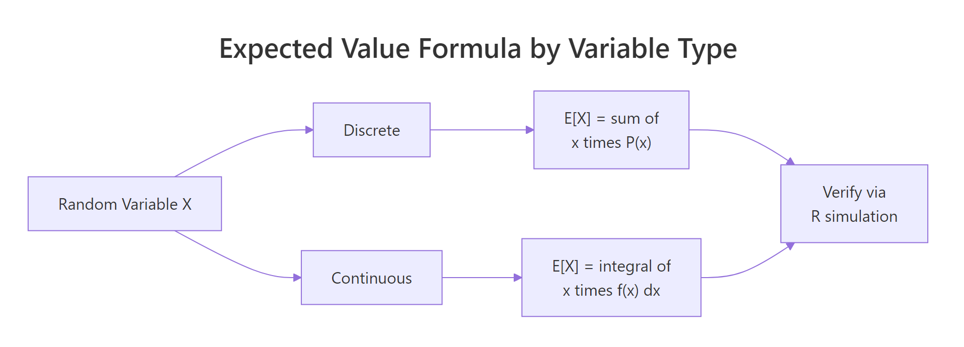
Figure 1: Discrete variables sum probability-weighted values; continuous variables integrate over the density. Either way, R simulation gives you a check in seconds.
Let us verify two classics: the uniform and the exponential.
Theoretical E = 0.5, sample mean = 0.5006. Theoretical Var = 0.0833, sample variance = 0.0834. Same pattern: one line of code delivers the numbers the integral would give you with more work.
Now an exponential distribution, which is skewed rather than flat.
Both statistics land inside 0.002 of the theoretical values. The exponential is a skewed distribution, most draws are near zero, with a long right tail, yet the machinery is exactly the same. Write down the formula, simulate, compare.
dexp(), pexp(), and rexp() take a rate parameter, not a mean. Many textbooks parameterize exponentials by mean $\beta = 1/\lambda$. If someone tells you "mean 10 exponential," use rate = 1/10 in R. Getting this backwards is the most common mistake with the exponential family.Try it: Compute theoretical $E[X]$ and $\text{Var}(X)$ for $X \sim \text{Uniform}(2, 10)$. Then simulate 10,000 draws and compare.
Click to reveal solution
Explanation: The uniform distribution is symmetric, so the mean is the midpoint. The variance depends only on the range, because shifting $(a, b)$ left or right does not change spread.
How do linearity and independence change E and Var?
Three rules do most of the practical work. Linearity of expectation. Quadratic scaling of variance. Additivity under independence. You can derive each from the definitions, but it is faster to state them and prove them by simulation.
Linearity of expectation (no independence assumption needed): $$E[aX + b] = a \cdot E[X] + b \qquad E[X + Y] = E[X] + E[Y]$$
Variance under linear transformation and independent sums: $$\text{Var}(aX + b) = a^2 \cdot \text{Var}(X) \qquad \text{Var}(X + Y) = \text{Var}(X) + \text{Var}(Y) \text{ if } X \perp Y$$
The $b$ drops out of variance because shifting every outcome by a constant does not change spread. The $a$ squares because variance is in squared units. Let us verify with dice.
The transformed variable has mean 15.5 and variance 26.25, right on the theoretical predictions. Notice the constant 5 lifted the mean by 5 but did not change the variance. The factor 3 scaled the mean by 3 and the variance by 9. That quadratic behavior is why standard deviation ($\sqrt{\text{Var}}$) is often the more intuitive spread measure, it scales linearly.
Now contrast independent versus correlated sums.
Two independent standard normals each have variance 1. Adding them gives variance 2. But if you add a standard normal to itself, you get variance 4, not 2, because the "variance adds" rule requires independence. Doubling $X$ scales its variance by $2^2 = 4$.
Try it: For $X \sim N(0, 1)$, simulate $Y = 3X$. Report the sample mean and sample variance of $Y$.
Click to reveal solution
Explanation: Mean scales linearly (3 times 0 is still 0). Variance scales by $3^2 = 9$. Standard deviation scales by 3, so $Y$ has sd 3 and var 9, which matches.
Why does the sample mean converge to E[X]?
Every simulation above worked because of the Law of Large Numbers. As you take more and more draws, the sample mean converges to the expected value. Let us watch it happen in slow motion.
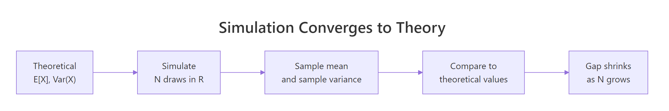
Figure 2: The gap between sample statistics and theoretical values shrinks as N grows. Simulation is a built-in check on every derivation you do.
Early on, the running mean swings wildly. With a handful of rolls, a few 6s in a row can pull it above 4. By N = 100 the curve has narrowed noticeably, and by N = 10,000 it is hugging 3.5 tightly. The variance of the sample mean shrinks as $\sigma^2 / N$, so its standard error shrinks as $\sigma / \sqrt{N}$.
Try it: Simulate a running mean for $X \sim \text{Poisson}(\lambda = 3)$ across N from 10 to 10,000. Plot it with a horizontal line at 3.
Click to reveal solution
Explanation: Poisson has $E[X] = \lambda = 3$, so the curve targets 3. The log-scale x-axis spreads out the early wild swings so you can see how the curve stabilizes.
Practice Exercises
Exercise 1: Custom discrete distribution
A random variable $X$ takes values 1, 2, 5, 10 with probabilities 0.4, 0.3, 0.2, 0.1. Compute $E[X]$ and $\text{Var}(X)$ by formula, then simulate 50,000 draws and confirm.
Click to reveal solution
Explanation: $E[X] = 1(0.4) + 2(0.3) + 5(0.2) + 10(0.1) = 3.0$. $E[X^2] = 1(0.4) + 4(0.3) + 25(0.2) + 100(0.1) = 16.6$, so $\text{Var}(X) = 16.6 - 3.0^2 = 7.6$. The simulated values land within 0.02 of both theoretical quantities, a tight match delivered by 50,000 draws.
Exercise 2: Verify variance via LOTUS
For $X \sim \text{Uniform}(0, 1)$, the Law of the Unconscious Statistician says $E[g(X)] = \int g(x) f(x) \, dx$. Use this to show $E[X^2] = 1/3$ analytically and by simulation. Then confirm the shortcut identity $\text{Var}(X) = E[X^2] - (E[X])^2 = 1/3 - 1/4 = 1/12$.
Click to reveal solution
Explanation: LOTUS says: to compute the expectation of a function of a random variable, average the function over the samples. You do not need the distribution of $g(X)$, just the distribution of $X$ itself. Both the direct var() and the shortcut identity agree with 1/12 to three decimal places.
Complete Example
Suppose your office logs the number of late arrivals per day over 300 weekdays. You want two things: the average expected daily lateness, and a measure of day-to-day variability. Here is the full loop, from raw counts to theoretical fit.
The empirical mean (2.49) and variance (2.62) are close, and their ratio is 1.05, very near the Poisson signature of 1. That suggests the count process is consistent with Poisson. If the ratio had been 3 or higher, the data would be overdispersed and you would reach for a negative binomial instead. Expected value and variance are not just textbook summaries, they are the first diagnostic you run on any count dataset.
Summary
The expected value is a weighted average and the variance is a weighted average of squared deviations. Everything else, continuous case, linearity, independence, is a variation on that theme. Simulation in R converts every formula into a visible, testable fact.
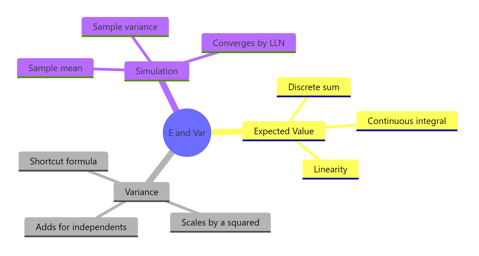
Figure 3: Expected value, variance, and simulation checks all connect through the same probability-weighted-average machinery.
| Concept | Formula | R code |
|---|---|---|
| Discrete E[X] | $\sum x \cdot P(x)$ | sum(vals * probs) |
| Continuous E[X] | $\int x \cdot f(x) \, dx$ | mean(sample) on a large simulated sample |
| Shortcut Var | $E[X^2] - (E[X])^2$ | sum(vals^2 * probs) - sum(vals * probs)^2 |
| Sample var (unbiased) | $\frac{1}{n-1} \sum (x_i - \bar{x})^2$ | var(x) |
| Linearity | $E[aX + b] = aE[X] + b$ | same identity holds in R numerically |
| Variance scaling | $\text{Var}(aX + b) = a^2 \text{Var}(X)$ | var(a * x + b) returns $a^2 \cdot \text{var}(x)$ |
| Independent sum | $\text{Var}(X + Y) = \text{Var}(X) + \text{Var}(Y)$ | only if x and y are independent draws |
| Convergence | sample mean error shrinks as $\sigma / \sqrt{N}$ | watch cumsum(x) / seq_along(x) |
Reach for the formula when you need closed-form answers. Reach for simulation when the formula is hard, when you want a sanity check, or when you need to communicate an intuition. The two methods together are stronger than either alone.
References
- Grinstead, C. & Snell, J. L.: Introduction to Probability, Chapter 6: Expected Value and Variance. Free online at American Mathematical Society. Link
- Pishro-Nik, H.: Introduction to Probability, Statistics, and Random Processes, Section 4.1.2: Expected Value and Variance. Link
- Ross, S.: A First Course in Probability, 10th Edition, Chapter 7 (Properties of Expectation). Pearson.
- MIT OpenCourseWare 18.05: Class 5 Prep: Variance of Discrete Random Variables. Link
- R Core Team:
var()function documentation in thestatspackage. Link - Dalgaard, P.: Introductory Statistics with R, 2nd Edition, Chapter 2 (Probability and Distributions). Springer.
Continue Learning
- Random Variables in R: The discrete-vs-continuous distinction that sets the stage for every expectation formula above.
- Binomial and Poisson Distributions in R: Named distributions where $E[X]$ and $\text{Var}(X)$ have simple closed forms in terms of the parameters.
- Central Limit Theorem in R: Why the sample mean not only converges to $E[X]$ but does so with a predictable normal-shaped error distribution.