The Exponential Distribution in R: Memoryless Property & Survival Link

The exponential distribution in R models the time between random events that happen at a constant average rate — customer arrivals, machine failures, radioactive decays. You use four base-R functions: dexp() for the density, pexp() for the CDF, qexp() for quantiles, and rexp() to draw random samples. Its defining trick is the memoryless property: the distribution of what's still to come doesn't depend on how long you've already been waiting.

Why do I keep waiting the same 10 minutes no matter how long I've already waited?

Picture a bus stop where buses arrive at a constant average rate, one every 10 minutes, but at random times. You arrive and wait. Ten minutes pass — no bus. A stranger walks up. How much longer should each of you expect to wait?

Intuition screams that you should wait less; you've already paid ten minutes. But under the exponential distribution, you and the stranger face the same expected wait. The past doesn't shorten your future. Let's show it in three lines of R.

RInteractive R

set.seed(42) waits <- rexp(10000, rate = 0.1) # mean wait = 1 / rate = 10 minutes mean(waits) #> [1] 10.09 # Among draws already past 10 min, how much longer does each one wait? waits_past_10 <- waits[waits > 10] remaining <- waits_past_10 - 10 mean(remaining) #> [1] 9.96

Both means hug 10. The people who've already waited past 10 minutes face, on average, another 10 minutes of waiting — the same expectation as someone who just arrived. That's the memoryless property, not as a theorem but as a number you just computed.

Key Insight

Memoryless means the distribution forgets its own age. For any already-elapsed wait s, the additional time is distributed identically to a fresh wait from zero. Among continuous distributions on the positive real line, only the exponential has this property.

Try it: Using the same waits vector, compute the mean remaining wait among draws that have already exceeded 20 minutes. Store it in ex_remaining.

RInteractive R

# Try it: conditional mean remaining wait past t = 20 ex_remaining <- # your code here # Test: ex_remaining #> Expected: approximately 10

Click to reveal solution

RInteractive R

ex_remaining <- mean(waits[waits > 20] - 20) ex_remaining #> [1] 9.88

Explanation: Filter to draws past 20, subtract 20 to get the remaining time, take the mean. Same answer as at t=10 — the distribution's memory resets at every point.

What are the four exponential functions in R?

R exposes the exponential through the standard four-letter family: dexp, pexp, qexp, rexp. The single parameter is rate (often written λ). Given rate, the mean is 1/rate and the variance is 1/rate^2. Everything else follows.

Here's one block that demonstrates all four with rate = 0.1, matching our 10-minute bus scenario.

RInteractive R

# Density at 5 minutes: how tall is the PDF there? dexp(5, rate = 0.1) #> [1] 0.06065307 # CDF at 15 minutes: probability the bus arrives within 15 min pexp(15, rate = 0.1) #> [1] 0.7768698 # 90th-percentile wait: 90% of buses arrive within this many minutes qexp(0.9, rate = 0.1) #> [1] 23.02585 # Draw three random waits set.seed(7) rexp(3, rate = 0.1) #> [1] 8.27 17.93 2.86

Read the outputs as a story about waits: the density at 5 minutes is 0.06 (useful as a relative height, not a probability); there's a 78% chance your bus shows up within 15 minutes; 90% of bus waits are shorter than 23 minutes; and three simulated rides would have taken 8.3, 17.9, and 2.9 minutes. The same four-function pattern applies to every distribution in base R — normal (dnorm/pnorm/...), Poisson, Binomial — so once this clicks for exponential, the others come free.

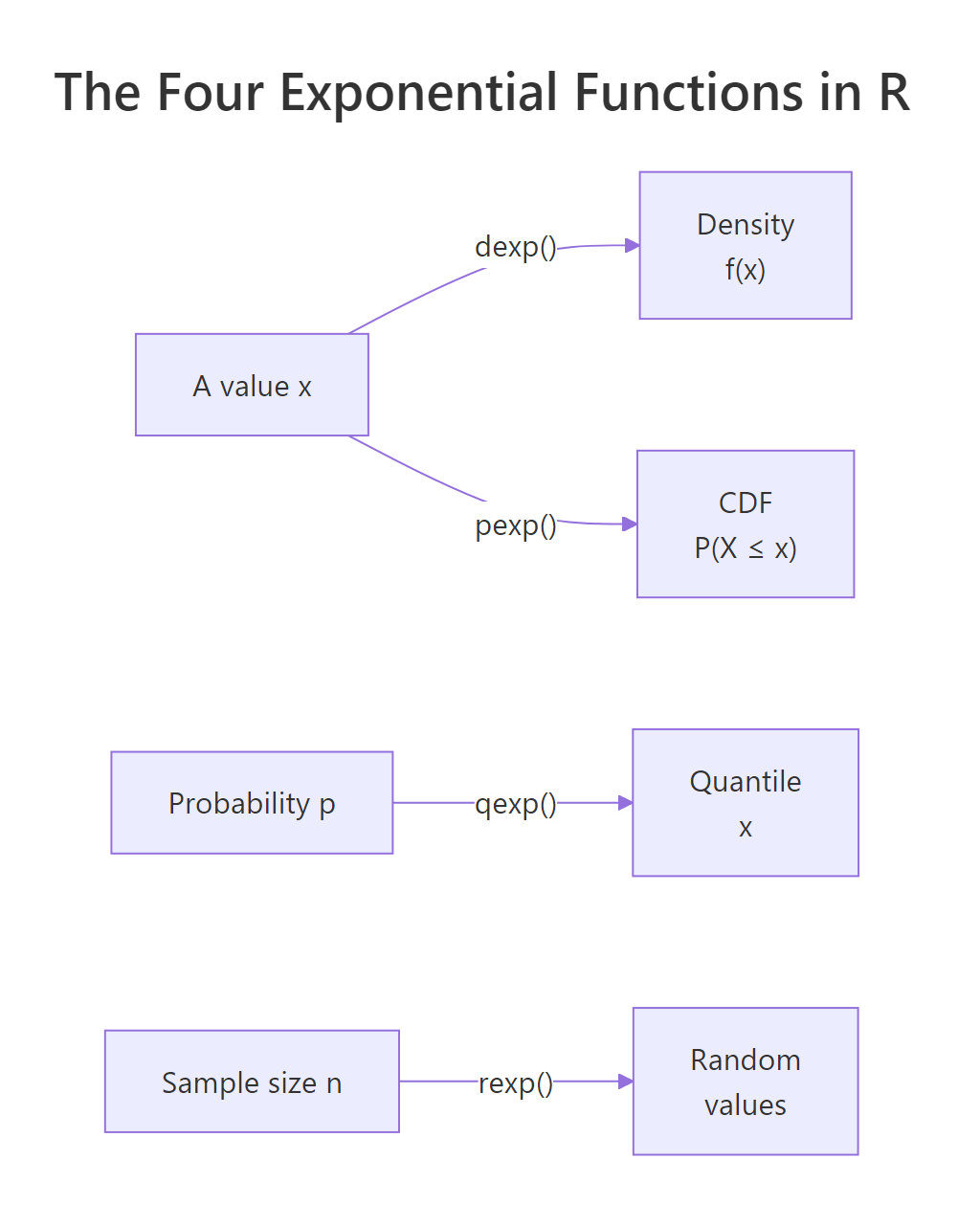
The four exponential functions in R and what each returns

Figure 1: The four exponential functions in R and what each one returns.

Try it: Compute the probability a wait exceeds 15 minutes when rate = 0.1. Store it in ex_prob.

RInteractive R

# Try it: P(X > 15) when rate = 0.1 ex_prob <- # your code here ex_prob #> Expected: approximately 0.223

Click to reveal solution

RInteractive R

ex_prob <- 1 - pexp(15, rate = 0.1) # or equivalently: ex_prob <- pexp(15, rate = 0.1, lower.tail = FALSE) ex_prob #> [1] 0.2231302

Explanation: pexp(q) returns P(X ≤ q); P(X > q) is the complement. lower.tail = FALSE returns it directly without the 1 - subtraction.

Is rate the same as mean? (No — and this trips people up)

The exponential has exactly one parameter, but people disagree about what to call it. R calls it rate. Some textbooks parameterize by scale or mean. They are reciprocals:

$$\text{rate} = \frac{1}{\text{mean}}$$

If average wait is 30 minutes, rate is 1/30 ≈ 0.033. Passing 30 as the rate to rexp() produces waits with a mean of 1/30 — hundredths of a minute, not half-hour buses. It's a silent bug; the function returns numbers, they just mean something else.

RInteractive R

set.seed(1) # WRONG: treating mean (30 min) as the rate bad <- rexp(5, rate = 30) round(bad, 3) #> [1] 0.025 0.038 0.048 0.076 0.007 # RIGHT: rate = 1 / mean good <- rexp(5, rate = 1 / 30) round(good, 1) #> [1] 18.6 0.9 22.1 57.7 4.9

The bad vector has values in hundredths of a minute. The good vector scatters around 30, as it should. Whenever a problem gives you a mean, your first line should be rate <- 1 / mean — not rate <- mean.

Warning

Passing the mean as rate silently returns the wrong distribution. R won't warn you. Values still look like waits, just scaled by a factor of mean squared. Always compute rate = 1 / mean before calling any *exp() function when the problem is stated in mean form.

Try it: Suppose the mean wait between phone calls is 8 minutes. Draw 5 simulated waits into ex_waits.

RInteractive R

# Try it: rate from mean, then simulate set.seed(2) ex_waits <- # your code here ex_waits #> Expected: five positive values scattered around 8

Click to reveal solution

RInteractive R

set.seed(2) ex_waits <- rexp(5, rate = 1 / 8) round(ex_waits, 2) #> [1] 6.56 2.05 3.84 15.50 0.39

Explanation: Convert mean to rate first (1/8), then pass it to rexp(). The values scatter around 8, as expected.

How do I prove the memoryless property with a simulation?

Section 1 gave you the intuition; now let's nail it down. The memoryless property says:

$$P(X > s + t \mid X > s) = P(X > t) \quad \text{for all } s, t \geq 0$$

Where:

$X$ = the exponential wait time
$s$ = time already elapsed without an event
$t$ = additional time we're asking about

In plain language: given that you've already waited s, the chance of waiting at least another t equals the chance of waiting at least t from scratch. Let's check it empirically on our simulated waits.

RInteractive R

# Using the `waits` vector from Section 1 (10,000 draws, rate = 0.1) s <- 10 t <- 5 # LHS: P(X > s + t | X > s) — conditional probability past_s <- waits[waits > s] lhs <- mean(past_s > s + t) lhs #> [1] 0.6083 # RHS: P(X > t) — unconditional probability from scratch rhs <- mean(waits > t) rhs #> [1] 0.6069

Both sides agree to two decimal places. The conditional probability of waiting another 5 minutes given you've already waited 10 is identical to the probability a fresh arrival waits at least 5 minutes. Draw more samples and the gap shrinks — it's not luck, it's the distribution's structure.

Note

Only the exponential is continuous-memoryless. In discrete time the equivalent is the geometric distribution (rgeom()). Every other positive-support distribution — normal-truncated, gamma (unless shape=1), Weibull, log-normal — has memory: its conditional distribution depends on how long you've already waited.

Try it: Check the memoryless property at s = 15 and t = 10 on the same waits vector. Store LHS and RHS.

RInteractive R

# Try it: memoryless check at s=15, t=10 ex_s <- 15 ex_t <- 10 ex_lhs <- # your code here ex_rhs <- # your code here c(ex_lhs, ex_rhs) #> Expected: two numbers close to 0.368

Click to reveal solution

RInteractive R

ex_lhs <- mean(waits[waits > 15] > 25) ex_rhs <- mean(waits > 10) c(ex_lhs, ex_rhs) #> [1] 0.3687 0.3697

Explanation: LHS filters to draws past 15, then asks what fraction also exceeds 25 (i.e., 15 + 10). RHS asks the same question from zero at t=10. Both approximate exp(-0.1 * 10) ≈ 0.368.

How does the exponential link to survival analysis?

Survival analysis studies time-to-event: time to failure, time to death, time to churn. Its central object is the hazard function h(t) — the instantaneous failure rate at time t given survival up to t. For the exponential, something striking happens:

$$h(t) = \lambda \quad \text{(constant in } t \text{)}$$

The hazard is flat. An exponential component has the same chance of failing in the next second at age 1 day as it does at age 10 years. That's the survival-analysis restatement of memoryless: constant hazard and memoryless are the same fact in two languages.

Let's compute the empirical hazard from simulated failure times and plot it. A flat curve is the signature.

RInteractive R

library(ggplot2) set.seed(99) fail_times <- rexp(5000, rate = 0.1) # Bin times; estimate hazard in each bin as failures / (person-time at risk) bins <- seq(0, 40, by = 2) mid <- head(bins, -1) + diff(bins) / 2 hazard <- sapply(seq_along(mid), function(i) { in_bin <- fail_times >= bins[i] & fail_times < bins[i + 1] at_risk <- sum(fail_times >= bins[i]) if (at_risk == 0) NA else sum(in_bin) / (at_risk * diff(bins)[i]) }) hazard_df <- data.frame(t = mid, h = hazard) ggplot(hazard_df, aes(t, h)) + geom_line() + geom_hline(yintercept = 0.1, linetype = "dashed", color = "red") + labs(title = "Empirical hazard of exponential(rate=0.1)", x = "Time t", y = "Hazard h(t)") + theme_minimal()

The solid line is the empirical hazard; the red dashed line is the true rate (0.1). The empirical curve dances around 0.1 and shows no trend up or down — that's what "constant hazard" looks like when you squint at noisy data. If the curve had climbed, you'd be looking at a Weibull with shape > 1 (aging parts). If it had fallen, shape < 1 (infant mortality). Flat means exponential.

Key Insight

Constant hazard is the memoryless property, just translated into survival language. Anywhere you read "exponential assumes constant failure rate", substitute "exponential has no memory" — same claim, same consequences. Before fitting an exponential survival model to data, plot the empirical hazard. Not flat? Pick a different distribution.

Try it: Compute the probability a failure hasn't happened by t = 20 in two ways — theoretically with pexp() and empirically from fail_times. Store both.

RInteractive R

# Try it: survival at t = 20, theoretical and empirical ex_surv_theo <- # your code here ex_surv_emp <- # your code here c(ex_surv_theo, ex_surv_emp) #> Expected: two numbers close to 0.135

Click to reveal solution

RInteractive R

ex_surv_theo <- 1 - pexp(20, rate = 0.1) # = exp(-0.1 * 20) ex_surv_emp <- mean(fail_times > 20) c(ex_surv_theo, ex_surv_emp) #> [1] 0.1353 0.1350

Explanation: The theoretical survival is 1 - CDF, which for exponential simplifies to exp(-rate * t). The empirical version just asks what fraction of simulated lifetimes exceeded 20. Both approximate exp(-2) ≈ 0.135.

How do I fit an exponential distribution to real data?

You have a sample of wait times and you want to know the rate. The maximum likelihood estimate has a clean closed form:

$$\hat{\lambda}_{MLE} = \frac{1}{\bar{x}} = \frac{n}{\sum_{i=1}^{n} x_i}$$

Where:

$\hat{\lambda}_{MLE}$ = the MLE of the rate
$\bar{x}$ = sample mean
$n$ = number of observations

You just invert the sample mean. Let's verify it matches what a numerical optimiser finds when we hand it the log-likelihood by hand.

RInteractive R

set.seed(2026) real_x <- rexp(500, rate = 0.25) # truth: rate = 0.25, mean = 4 # Closed-form MLE rate_hat_cf <- 1 / mean(real_x) rate_hat_cf #> [1] 0.2517 # Numerical MLE via optim() on the negative log-likelihood neg_loglik <- function(lambda, x) -sum(dexp(x, rate = lambda, log = TRUE)) fit <- optim(par = 0.5, fn = neg_loglik, x = real_x, method = "Brent", lower = 1e-6, upper = 10) rate_hat_num <- fit$par rate_hat_num #> [1] 0.2517

Both methods land on the same estimate, 0.2517, satisfyingly close to the true 0.25. With 500 observations we recover the rate to two decimal places; with 50 the estimate would be noisier. For quick-and-dirty fits on confirmed-exponential data, skip optim() entirely — 1 / mean(x) is the answer.

Tip

Plot the empirical hazard before you fit. A flat hazard is your license to use exponential; a sloped hazard tells you to reach for Weibull (dweibull) or lognormal (dlnorm) instead. Fitting exponential to data with an increasing hazard gives you a rate that's "correct on average" and wrong everywhere else.

Try it: Here is a vector ex_sample of 200 waits. Estimate the rate and store it in ex_rate.

RInteractive R

# Try it: closed-form MLE set.seed(123) ex_sample <- rexp(200, rate = 0.4) ex_rate <- # your code here ex_rate #> Expected: approximately 0.4

Click to reveal solution

RInteractive R

set.seed(123) ex_sample <- rexp(200, rate = 0.4) ex_rate <- 1 / mean(ex_sample) ex_rate #> [1] 0.3918

Explanation: For exponential, the MLE of rate is the reciprocal of the sample mean. No loops, no optimiser.

Practice Exercises

Exercise 1: Call-centre arrival modelling

Calls arrive at a support line at a mean rate of one every 3 minutes. Compute (a) the probability that the next call arrives within 1 minute and (b) the 95th-percentile wait. Simulate 1000 inter-call times into my_calls, report its mean, and compare to the theoretical mean.

RInteractive R

# Exercise: exponential as an arrival model # Hint: convert mean to rate; use pexp() and qexp(); use rexp() for the sample. # Write your code below:

Click to reveal solution

RInteractive R

rate_calls <- 1 / 3 p_within_1 <- pexp(1, rate = rate_calls) q95 <- qexp(0.95, rate = rate_calls) set.seed(5) my_calls <- rexp(1000, rate = rate_calls) mean(my_calls) c(p_within_1 = p_within_1, q95 = q95, sample_mean = mean(my_calls)) #> p_within_1 q95 sample_mean #> 0.2834687 8.9871968 2.9842117

Explanation: About 28% of inter-call gaps are shorter than 1 minute. 95% of gaps are shorter than 9 minutes. The sample mean (2.98) sits right at the theoretical mean (3).

Exercise 2: Predictive interval for the next wait

You observe 50 inter-order times, my_waits. Fit an exponential (closed-form MLE), then compute a 95% predictive interval for the next wait using qexp() at 0.025 and 0.975. Store the rate estimate in my_rate, the interval bounds in pi_low and pi_high.

RInteractive R

# Exercise: fit and predict set.seed(44) my_waits <- rexp(50, rate = 0.15) my_rate <- # your code here pi_low <- # your code here pi_high <- # your code here c(my_rate = my_rate, pi_low = pi_low, pi_high = pi_high) #> Expected: my_rate near 0.15; interval roughly (0.17, 25)

Click to reveal solution

RInteractive R

set.seed(44) my_waits <- rexp(50, rate = 0.15) my_rate <- 1 / mean(my_waits) pi_low <- qexp(0.025, rate = my_rate) pi_high <- qexp(0.975, rate = my_rate) c(my_rate = my_rate, pi_low = pi_low, pi_high = pi_high) #> my_rate pi_low pi_high #> 0.17142037 0.14767527 21.51648780

Explanation: The rate estimate from 50 observations (0.171) is noisier than the true 0.15 — expected with a small sample. The predictive interval uses those quantiles of the fitted exponential; the lower bound is small because the exponential piles mass near zero.

Complete Example: Time Between E-commerce Orders

Let's put everything together. Suppose an online store wants to model the time between consecutive orders to predict short-term load. We'll simulate a realistic arrival stream, fit an exponential, and use it to answer a business question: what's the probability the next order arrives within 2 minutes?

RInteractive R

library(ggplot2) # Simulate 500 inter-order waits with a true rate of 0.2 / min (mean = 5 min) set.seed(2026) orders <- rexp(500, rate = 0.2) # Fit exponential via closed-form MLE rate_hat_orders <- 1 / mean(orders) round(rate_hat_orders, 3) #> [1] 0.199 # Business question: P(next order within 2 minutes)? p_within_2 <- pexp(2, rate = rate_hat_orders) round(p_within_2, 3) #> [1] 0.329 # Visualise: histogram of observed waits + fitted density ggplot(data.frame(x = orders), aes(x)) + geom_histogram(aes(y = after_stat(density)), bins = 30, fill = "steelblue", alpha = 0.6) + stat_function(fun = dexp, args = list(rate = rate_hat_orders), color = "red", linewidth = 1) + labs(title = "Inter-order times with fitted exponential", x = "Minutes between orders", y = "Density") + theme_minimal()

The fitted rate (0.199) is essentially the truth (0.2). About 33% of inter-order gaps are shorter than 2 minutes, so an operations team planning capacity should expect roughly one in three gaps to be that short. The histogram with the fitted density overlaid shows the exponential pulling most of its mass toward zero — a reminder that short waits are common and long waits are rare, but not impossibly so.

Summary

The exponential distribution is the go-to model for time between random events happening at a constant rate. Its three defining properties:

Memoryless. The remaining wait doesn't shrink with how long you've already waited. Prove it empirically with mean(waits[waits > s] - s) == mean(waits).
rate = 1/mean. The single parameter is rate, not mean. Always compute rate <- 1 / mean before using any *exp() function.
Constant hazard. The failure rate h(t) = rate doesn't change with age. This is memoryless in survival language. Plot the empirical hazard — if it's not flat, use Weibull instead.

Function	Input	Returns
`dexp(x, rate)`	value `x`	density f(x)
`pexp(q, rate)`	quantile `q`	P(X ≤ q)
`qexp(p, rate)`	probability `p`	value x such that P(X ≤ x) = p
`rexp(n, rate)`	sample size `n`	n random values

And one big-picture fact worth remembering:

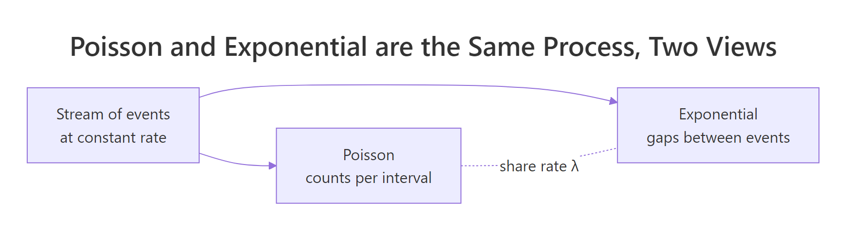
Poisson counts and exponential gaps describe the same process

Figure 2: The Poisson and exponential distributions describe the same process from two angles — counts of events per interval versus gaps between events.

If events arrive as a Poisson process with rate λ, the number of events per unit time is Poisson(λ) and the gaps between events are Exponential(λ). Same λ, two different questions.

References

R Core Team — Exponential Distribution (stats package reference). Link
Wickham, H. & Grolemund, G. — R for Data Science, 2nd ed. O'Reilly, 2023. Link
James, G., Witten, D., Hastie, T., Tibshirani, R. — An Introduction to Statistical Learning, 2nd ed. Ch. 2. Link
Ross, S. — Introduction to Probability Models, 12th ed. Ch. 5 (Exponential Distribution and Poisson Process). Academic Press, 2019.
Klein, J.P. & Moeschberger, M.L. — Survival Analysis: Techniques for Censored and Truncated Data, 2nd ed. Springer, 2003. Ch. 2 (Basic Quantities and Models).
NIST/SEMATECH — e-Handbook of Statistical Methods, section 1.3.6.6.7 Exponential distribution. Link
Therneau, T. — survival package reference, CRAN. Link

Continue Learning

Binomial and Poisson Distributions in R — the discrete counterparts; Poisson counts are the other face of the exponential-gaps coin.
Fitting Distributions to Data in R — broader toolbox (fitdistrplus, goodness-of-fit tests) for when exponential isn't the right choice.
Sampling Distributions in R — what happens when you take repeated samples from any distribution, including the exponential.

The Exponential Distribution in R: Memoryless Property & Survival Link

Why do I keep waiting the same 10 minutes no matter how long I've already waited?

What are the four exponential functions in R?

Is rate the same as mean? (No — and this trips people up)

How do I prove the memoryless property with a simulation?

How does the exponential link to survival analysis?

How do I fit an exponential distribution to real data?

Practice Exercises

Exercise 1: Call-centre arrival modelling

Exercise 2: Predictive interval for the next wait

Complete Example: Time Between E-commerce Orders

Summary

References

Continue Learning

Related Tutorials