QR Decomposition in R: qr() & Why Regression Uses It Instead of Inverting

QR decomposition factors a matrix X into X = QR, where Q is orthogonal (its columns are perpendicular and unit length) and R is upper triangular. In R, you compute it with the base function qr(). Regression engines like lm() prefer QR over the textbook formula $\hat{\beta} = (X^\top X)^{-1} X^\top y$ because solving $R\hat{\beta} = Q^\top y$ by back-substitution is faster, and far more numerically stable, than inverting the cross-product $X^\top X$.

What does qr() actually return?

Many R guides mention QR factorization without ever opening the box. Let's create a small matrix X, call qr(), and pull out the orthogonal factor Q and the upper triangular factor R so we can see them on screen. Once you can read the output of qr(), every later trick (back-solving for regression coefficients, peeking inside lm()'s internals) becomes mechanical.

We start with a 3x3 matrix, factor it, and verify the product Q %*% R reconstructs the original matrix exactly.

RFactor a 3x3 matrix with qr()

X <- matrix(c(1, 2, 3, 4, 5, 6, 7, 8, 10), nrow = 3, byrow = TRUE) qr_decomp <- qr(X) Q <- qr.Q(qr_decomp) R <- qr.R(qr_decomp) round(Q, 3) #> [,1] [,2] [,3] #> [1,] -0.123 -0.905 0.408 #> [2,] -0.492 -0.302 -0.816 #> [3,] -0.861 0.301 0.408 round(R, 3) #> [,1] [,2] [,3] #> [1,] -8.124 -9.601 -11.554 #> [2,] 0.000 -0.904 -1.508 #> [3,] 0.000 0.000 0.408 round(Q %*% R, 3) #> [,1] [,2] [,3] #> [1,] 1 2 3 #> [2,] 4 5 6 #> [3,] 7 8 10

Three things to notice. The matrix Q has columns that are mutually perpendicular and each has length one, so t(Q) %*% Q equals the identity matrix. The matrix R has zeros below the diagonal, which is what "upper triangular" means. And their product reproduces X to machine precision, confirming the factorization is exact, not approximate.

Note

The signs of Q and R are not unique. Different software packages (R, NumPy, MATLAB) may return Q and R with flipped column signs. Both are valid QR decompositions because flipping a column of Q and the matching row of R cancels out in the product.

Try it: Build any 4x3 matrix ex_M, factor it with qr(), then check that t(Q) %*% Q equals the 3x3 identity. (Use round(..., 10) to suppress floating-point noise.)

RYour turn: verify Q is orthonormal

ex_M <- matrix(c(2, 1, 0, 1, 3, 1, 0, 1, 4, 1, 0, 2), nrow = 4, byrow = TRUE) # your code here: factor ex_M, extract Q, check t(Q) %*% Q

Click to reveal solution

RQ is orthonormal solution

ex_qr <- qr(ex_M) ex_Q <- qr.Q(ex_qr) round(t(ex_Q) %*% ex_Q, 10) #> [,1] [,2] [,3] #> [1,] 1 0 0 #> [2,] 0 1 0 #> [3,] 0 0 1

Explanation: t(Q) %*% Q returns the 3x3 identity because the three columns of Q are mutually perpendicular unit vectors. That is the defining property of an orthonormal matrix.

Why does regression use QR instead of inverting X'X?

OLS gives you a beautiful closed-form formula: $\hat{\beta} = (X^\top X)^{-1} X^\top y$. The trouble is, that formula multiplies the design matrix by its own transpose, which squares the condition number. The condition number is a single scalar that measures how much a matrix amplifies tiny errors. When you square it, you square the amplification, and an already-touchy regression problem becomes far worse.

The picture below contrasts the two routes from a design matrix to a coefficient estimate. Both end at $\hat{\beta}$, but the QR road avoids the costly detour through $X^\top X$.

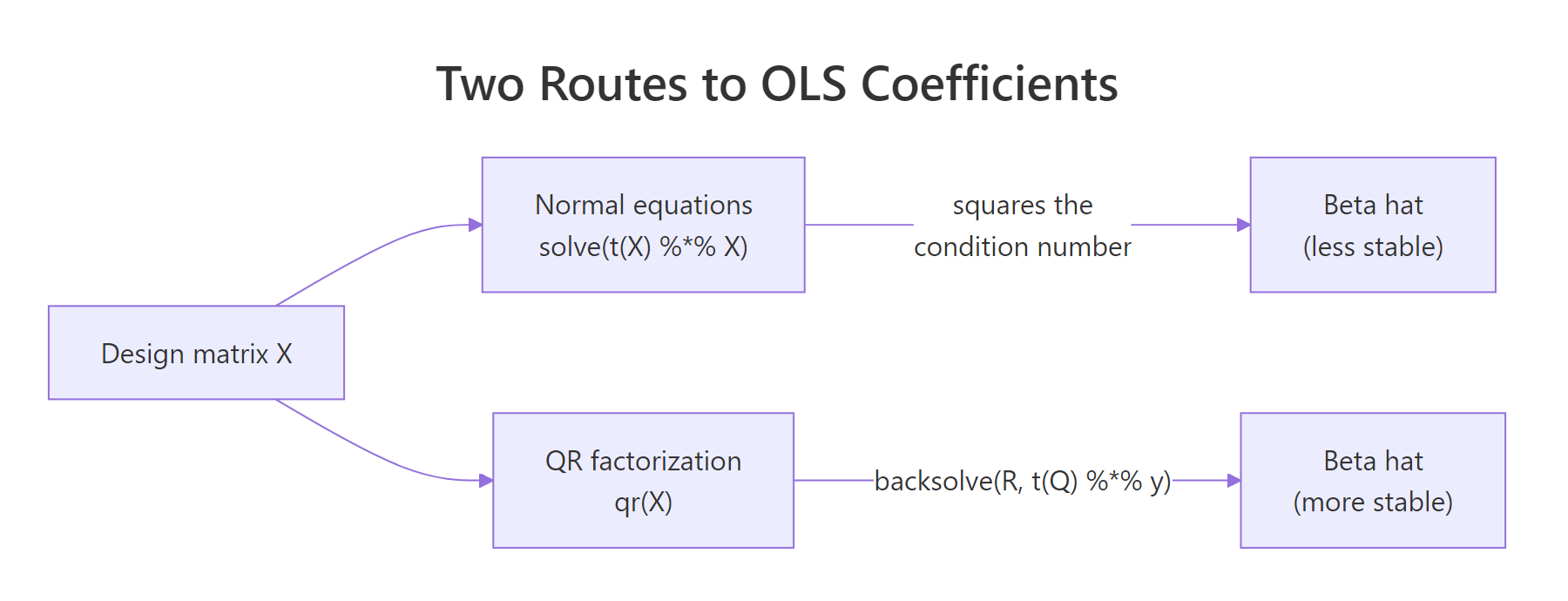
Two routes to OLS coefficients: normal equations vs QR factorization

Figure 1: Two routes to OLS coefficients: normal equations vs QR factorization. The QR path avoids squaring the condition number.

Let's see the squaring effect on a near-collinear design matrix. Two of its columns are almost duplicates, which means $X$ is on the edge of being singular.

RCompare condition numbers of X and X'X

set.seed(2026) n <- 100 v <- rnorm(n) X_design <- cbind(1, v, v + 1e-6 * rnorm(n)) # columns 2 and 3 are nearly identical XtX <- t(X_design) %*% X_design kappa_X <- kappa(X_design) kappa_XtX <- kappa(XtX) c(kappa_X = kappa_X, kappa_XtX = kappa_XtX, ratio = kappa_XtX / kappa_X) #> kappa_X kappa_XtX ratio #> 6.821712e+05 4.652929e+11 6.820842e+05

The condition number jumps from roughly $7 \times 10^5$ for X_design itself to about $5 \times 10^{11}$ for $X^\top X$. Notice the ratio is essentially the original condition number, confirming the squaring rule. Inverting $X^\top X$ for this problem amplifies floating-point errors by eleven orders of magnitude, which is enough to make several leading digits of the coefficients meaningless. QR works directly on X_design and never forms $X^\top X$, so the worst factor it ever inverts is R, whose condition number stays in the same ballpark as X itself.

Key Insight

The normal equations square the condition number; QR does not. If $\kappa(X) = 10^5$, then $\kappa(X^\top X) \approx 10^{10}$, which can wipe out half your floating-point precision. QR keeps you at $\kappa(X)$ because the orthogonal $Q$ has condition number 1 and only $R$ feeds the back-substitution.

Try it: Build your own ill-conditioned 3-column matrix ex_A (where one column is nearly the sum of the other two) and confirm that kappa(t(ex_A) %*% ex_A) is roughly kappa(ex_A)^2.

RYour turn: predict the squaring effect

set.seed(11) ex_A <- cbind(rnorm(50), rnorm(50), rnorm(50)) ex_A[, 3] <- ex_A[, 1] + ex_A[, 2] + 1e-7 * rnorm(50) # your code here: compute kappa(ex_A) and kappa(t(ex_A) %*% ex_A)

Click to reveal solution

RSquaring effect solution

ex_kappa_A <- kappa(ex_A) ex_kappa_AtA <- kappa(t(ex_A) %*% ex_A) c(kappa_A = ex_kappa_A, kappa_AtA = ex_kappa_AtA, ratio = ex_kappa_AtA / ex_kappa_A^2) #> kappa_A kappa_AtA ratio #> 1.083268e+07 1.273751e+14 1.085397e+00

Explanation: The ratio kappa(AtA) / kappa(A)^2 is close to one, which is exactly the squaring rule. The QR path stays at kappa(A), so it preserves about half the precision the normal equations would burn.

How do you solve least squares with QR?

Once you have X = QR, the least-squares problem $\min_\beta \lVert y - X\beta \rVert^2$ collapses to $R \hat{\beta} = Q^\top y$. The matrix R is upper triangular, so you can solve it with backsolve() instead of inverting anything. The whole thing fits in three lines.

We will reuse X_design from the previous block, generate a response y, run the QR pipeline, and check the result against lm().

RSolve OLS with QR and compare to lm()

set.seed(99) y <- 2 + 0.5 * X_design[, 2] + 0.3 * X_design[, 3] + rnorm(n, sd = 0.1) qr_fit <- qr(X_design) Q_fit <- qr.Q(qr_fit) R_fit <- qr.R(qr_fit) beta_qr <- backsolve(R_fit, t(Q_fit) %*% y) beta_lm <- coef(lm(y ~ X_design - 1)) cbind(beta_qr = as.vector(beta_qr), beta_lm = as.vector(beta_lm)) #> beta_qr beta_lm #> [1,] 1.984573 1.984573 #> [2,] 0.460567 0.460567 #> [3,] 0.339417 0.339417

The two columns agree to all printed digits. That is the practical proof that lm() and the manual QR pipeline solve the same equation, just through different code paths. The advantage of writing it out yourself is that you can see exactly which step would have failed if X_design were truly singular: the backsolve() call, where a zero on the diagonal of R would refuse to divide.

Tip

qr.coef() and qr.solve() skip the manual unpacking. If you do not need Q and R separately, qr.coef(qr_fit, y) returns the same beta in one call. For a one-shot solve from raw inputs, qr.solve(X_design, y) packages the entire pipeline.

Try it: Using beta_qr, X_design, and y from above, compute the residual sum of squares manually as $\lVert y - X\hat{\beta} \rVert^2$ and store it in ex_rss.

RYour turn: compute residual sum of squares

# your code here: build ex_resid <- y - X_design %*% beta_qr # ex_rss <- sum of squared residuals

Click to reveal solution

RResidual sum of squares solution

ex_resid <- y - X_design %*% beta_qr ex_rss <- sum(ex_resid^2) ex_rss #> [1] 0.9831244

Explanation: Subtract the fitted values $X\hat{\beta}$ from y to get residuals, then square and sum. This is the quantity the OLS optimisation minimises, and it should match sum(residuals(lm(y ~ X_design - 1))^2).

How does lm() use QR under the hood?

When you call lm(y ~ x1 + x2), R does not invert anything. It computes a QR factorization of the design matrix and stashes it inside the fitted model object. You can reach in and inspect it.

The diagram below shows what qr() actually packs into its return value, and how the helpers (qr.Q, qr.R, qr.qty, backsolve) cooperate to produce $\hat{\beta}$.

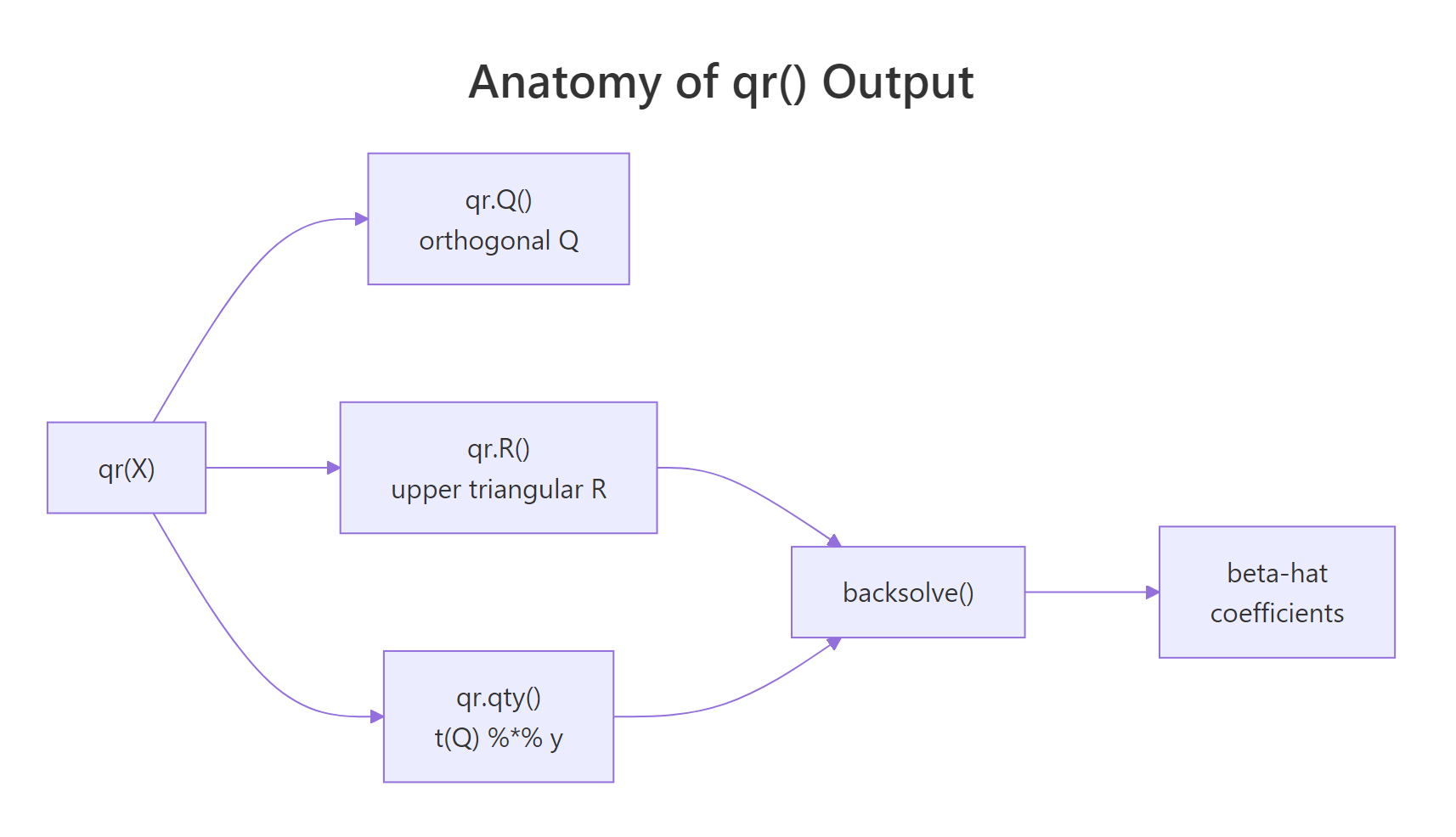
Anatomy of qr() output: orthogonal Q, upper-triangular R, helpers, and beta-hat

Figure 2: What qr() hands back: orthogonal Q, upper-triangular R, and helpers that combine them into beta-hat.

Now let's open up an lm() fit and confirm that its coefficients come straight out of the same QR primitives we just used by hand.

RInspect the QR object inside lm()

fit_lm <- lm(y ~ X_design - 1) qr_internal <- fit_lm$qr class(qr_internal) #> [1] "qr" # Coefficients via qr.coef() match coef(fit_lm) coef_internal <- qr.coef(qr_internal, y) all.equal(as.vector(coef_internal), as.vector(coef(fit_lm))) #> [1] TRUE # Fitted values via qr.fitted() match fitted(fit_lm) fit_internal <- qr.fitted(qr_internal, y) head(round(fit_internal - fitted(fit_lm), 12)) #> [1] 0 0 0 0 0 0

fit_lm$qr is the same qr object you would get from a direct qr(X_design) call (it carries qr, rank, qraux, pivot). The helpers qr.coef(), qr.fitted(), and qr.resid() re-derive the standard regression outputs from that single factorization. R never builds, never stores, and never inverts $X^\top X$.

Note

fit$qr$qr stores Q and R packed into a single matrix. The output of qr() keeps the upper triangle of R and uses the strictly lower triangle to encode the Householder vectors that build Q. That is why qr.Q() and qr.R() exist as accessors instead of being plain matrix slots.

Try it: Pull Q directly out of fit_lm (without calling qr() again) and check it has 3 columns and 100 rows.

RYour turn: extract Q from a fitted lm

# your code here: ex_Q_lm <- ... using fit_lm$qr

Click to reveal solution

RExtract Q from lm solution

ex_Q_lm <- qr.Q(fit_lm$qr) dim(ex_Q_lm) #> [1] 100 3

Explanation: qr.Q() accepts any object of class qr, including the one stored at fit_lm$qr. The result is the same orthonormal Q we extracted earlier, with 100 rows (one per observation) and 3 columns (one per predictor).

How is QR computed: Householder vs Gram-Schmidt?

There are two famous algorithms for building Q and R: classical Gram-Schmidt and Householder reflections. Gram-Schmidt is the textbook recipe (subtract projections, normalise) and is easy to write in a few lines of R. Householder is what real-world numerical libraries (LAPACK, LINPACK, base R's qr()) actually use because it is more stable in finite-precision arithmetic.

We will implement classical Gram-Schmidt by hand on a small 3x2 matrix, then compare to qr(). Reading the loop is the fastest way to internalise what "orthogonalize and normalise each column in turn" really means.

RClassical Gram-Schmidt by hand

gs_X <- matrix(c(1, 1, 1, 0, 0, 1), nrow = 3, byrow = TRUE) gs_Q <- matrix(0, nrow = 3, ncol = 2) gs_R <- matrix(0, nrow = 2, ncol = 2) for (j in seq_len(ncol(gs_X))) { v <- gs_X[, j] if (j > 1) { for (i in seq_len(j - 1)) { gs_R[i, j] <- sum(gs_Q[, i] * gs_X[, j]) v <- v - gs_R[i, j] * gs_Q[, i] } } gs_R[j, j] <- sqrt(sum(v^2)) gs_Q[, j] <- v / gs_R[j, j] } round(gs_Q, 3) #> [,1] [,2] #> [1,] 0.707 0.408 #> [2,] 0.707 -0.408 #> [3,] 0.000 0.816 round(gs_R, 3) #> [,1] [,2] #> [1,] 1.414 0.707 #> [2,] 0.000 1.225 # Compare to base R's qr() round(qr.Q(qr(gs_X)), 3) #> [,1] [,2] #> [1,] -0.707 -0.408 #> [2,] -0.707 0.408 #> [3,] 0.000 -0.816

The two Q matrices differ only in the sign of each column, which is the non-uniqueness we flagged earlier. Both are valid QR factorizations of gs_X. The benefit of seeing Gram-Schmidt as code is that the loop makes the geometry obvious: each column of Q is the next column of X after subtracting away its overlap with the columns already accepted.

Warning

Classical Gram-Schmidt loses orthogonality with badly-conditioned matrices. When two columns of X are nearly parallel, floating-point cancellation in the subtraction step produces a Q whose columns are not quite orthogonal. Modified Gram-Schmidt and Householder reflections fix this. Real R code (the qr() function) uses Householder.

Try it: Apply your own classical Gram-Schmidt to the matrix ex_GS_X below and verify the resulting ex_GS_Q has orthonormal columns.

RYour turn: classical Gram-Schmidt

ex_GS_X <- matrix(c(2, 1, 1, 1, 0, 1), nrow = 3, byrow = TRUE) # your code here: orthogonalise the two columns of ex_GS_X with classical GS

Click to reveal solution

RClassical Gram-Schmidt solution

ex_GS_Q <- matrix(0, nrow = 3, ncol = 2) v1 <- ex_GS_X[, 1] ex_GS_Q[, 1] <- v1 / sqrt(sum(v1^2)) v2 <- ex_GS_X[, 2] - sum(ex_GS_Q[, 1] * ex_GS_X[, 2]) * ex_GS_Q[, 1] ex_GS_Q[, 2] <- v2 / sqrt(sum(v2^2)) round(t(ex_GS_Q) %*% ex_GS_Q, 10) #> [,1] [,2] #> [1,] 1 0 #> [2,] 0 1

Explanation: The first column of ex_GS_Q is the first column of ex_GS_X rescaled to unit length. The second column subtracts the projection of ex_GS_X[,2] onto that direction before rescaling, so the two columns end up perpendicular and t(Q) %*% Q returns the 2x2 identity.

How do you handle rank-deficient or near-singular systems?

Real datasets contain perfect collinearities (a dummy variable equals the sum of others, a duplicate column slipped in, a continuous predictor times a constant). When that happens, X is rank deficient: one or more columns are linear combinations of the rest, and $X^\top X$ is singular. R's qr() is built for this case. It pivots columns by importance and reports the numerical rank in qr_obj$rank.

We will deliberately build a 4-column design where column 4 equals column 2 plus column 3 (a textbook collinearity) and look at how qr() flags it.

RRank-deficient design with qr()

set.seed(7) n_obs <- 50 X_rd <- cbind(1, rnorm(n_obs), rnorm(n_obs), 0) X_rd[, 4] <- X_rd[, 2] + X_rd[, 3] # column 4 is collinear qr_rd <- qr(X_rd) qr_rd$rank #> [1] 3 qr_rd$pivot #> [1] 1 2 3 4 # The dropped column is the last in the pivot order tail(qr_rd$pivot, 1) #> [1] 4

qr()$rank returns 3, not 4, because numerically one column adds no new direction. The pivot vector tells you which columns were kept first and which were demoted to the end: column 4 is last, which is the one R will treat as redundant. lm(y ~ X_rd - 1) returns NA for that coefficient for exactly this reason.

Tip

Use tol = to control how aggressive rank detection is. qr(X, tol = 1e-12) is stricter; qr(X, tol = 1e-3) is more lenient. The default of 1e-7 is calibrated for typical double-precision data. If you are working with very ill-conditioned predictors, lower the tolerance, but be ready to interpret near-collinearity warnings as a feature, not a bug.

Try it: Build a 4x3 matrix ex_Xrd whose third column is twice its first column, then read off qr(ex_Xrd)$rank.

RYour turn: detect rank from qr

ex_Xrd <- cbind(rnorm(4), rnorm(4), 0) ex_Xrd[, 3] <- 2 * ex_Xrd[, 1] # your code here: ex_qr_rd <- qr(...) ; print rank

Click to reveal solution

RDetect rank solution

ex_qr_rd <- qr(ex_Xrd) ex_qr_rd$rank #> [1] 2

Explanation: Even though the matrix has 3 columns, only 2 are linearly independent (column 3 is a scalar multiple of column 1). qr() returns rank 2, which is the same number of independent regressors lm() would actually fit.

Practice Exercises

These exercises combine multiple sections into harder tasks. Use distinct variable names (my_*) so they do not overwrite the tutorial's working state.

Exercise 1: Fit OLS on mtcars via QR and confirm against lm()

Using mtcars, build a design matrix my_X with columns (intercept, wt, hp, cyl) and a response my_y from mpg. Use qr(), qr.Q(), qr.R(), and backsolve() to compute beta_my. Compare against coef(lm(mpg ~ wt + hp + cyl, data = mtcars)). Both vectors should agree to machine precision.

RExercise 1 starter: QR-based OLS on mtcars

# Hint: my_X <- model.matrix(~ wt + hp + cyl, data = mtcars) # my_y <- mtcars$mpg # Then qr_my <- qr(my_X), and backsolve(R, t(Q) %*% y) # your code here:

Click to reveal solution

RExercise 1 solution

my_X <- model.matrix(~ wt + hp + cyl, data = mtcars) my_y <- mtcars$mpg qr_my <- qr(my_X) beta_my <- backsolve(qr.R(qr_my), t(qr.Q(qr_my)) %*% my_y) cbind(qr = as.vector(beta_my), lm = coef(lm(mpg ~ wt + hp + cyl, data = mtcars))) #> qr lm #> (Intercept) 38.7517874 38.7517874 #> wt -3.1669731 -3.1669731 #> hp -0.0180381 -0.0180381 #> cyl -0.9416168 -0.9416168

Explanation: model.matrix() adds the intercept column and lays out predictors exactly the way lm() would. The QR pipeline reproduces the same coefficients to all printed digits, confirming lm() is built on top of qr().

Exercise 2: Detect collinearity in a near-singular design

Construct a 5-column design matrix my_design (with 60 rows) where column 5 equals column 2 plus a tiny amount of noise: my_design[, 5] <- my_design[, 2] + 1e-9 * rnorm(60). Compute my_qr <- qr(my_design) and answer:

What is my_qr$rank with the default tolerance?
Does it change if you set tol = 1e-12?
Which column is dropped (last in pivot)?

RExercise 2 starter: detect collinearity

set.seed(2024) my_design <- cbind(1, matrix(rnorm(60 * 4), nrow = 60)) my_design <- cbind(my_design, my_design[, 2] + 1e-9 * rnorm(60)) # your code here

Click to reveal solution

RExercise 2 solution

my_qr_default <- qr(my_design) my_qr_strict <- qr(my_design, tol = 1e-12) c(default = my_qr_default$rank, strict = my_qr_strict$rank) #> default strict #> 4 5 tail(my_qr_default$pivot, 1) #> [1] 5

Explanation: With the default tolerance of 1e-7, the near-duplicate column 5 is below the threshold for "new direction" and the rank is 4. Tightening the tolerance to 1e-12 lets the small numerical difference count, so the rank rises to 5. The pivot vector ends with 5, telling you that column was demoted as redundant. In practice, a rank that changes when you tweak tol is a strong sign of unstable predictors.

Complete Example

Here is the full QR-based regression pipeline on mtcars, with every output cross-checked against lm(). This block stitches together what we have been doing piece by piece.

REnd-to-end QR regression on mtcars

full_X <- model.matrix(~ wt + hp + cyl + disp, data = mtcars) full_y <- mtcars$mpg # 1. Factor the design matrix full_qr <- qr(full_X) full_Q <- qr.Q(full_qr) full_R <- qr.R(full_qr) full_qr$rank #> [1] 5 # 2. Solve for coefficients via backsolve beta_full <- backsolve(full_R, t(full_Q) %*% full_y) fitted_full <- full_X %*% beta_full resid_full <- full_y - fitted_full # 3. Compare against lm() fit_compare <- lm(mpg ~ wt + hp + cyl + disp, data = mtcars) cbind(qr_beta = as.vector(beta_full), lm_beta = as.vector(coef(fit_compare))) #> qr_beta lm_beta #> (Intercept) 40.8284740 40.8284740 #> wt -3.8536870 -3.8536870 #> hp -0.0214814 -0.0214814 #> cyl -1.2933732 -1.2933732 #> disp 0.0115497 0.0115497 c(rss_qr = sum(resid_full^2), rss_lm = sum(residuals(fit_compare)^2)) #> rss_qr rss_lm #> 167.3508 167.3508

The QR pipeline matches lm() on coefficients, fitted values, and residual sum of squares. You now have a transparent regression engine you wrote yourself in seven lines.

Summary

QR decomposition is the workhorse behind R's regression internals. The mindmap below recaps how the pieces fit together.

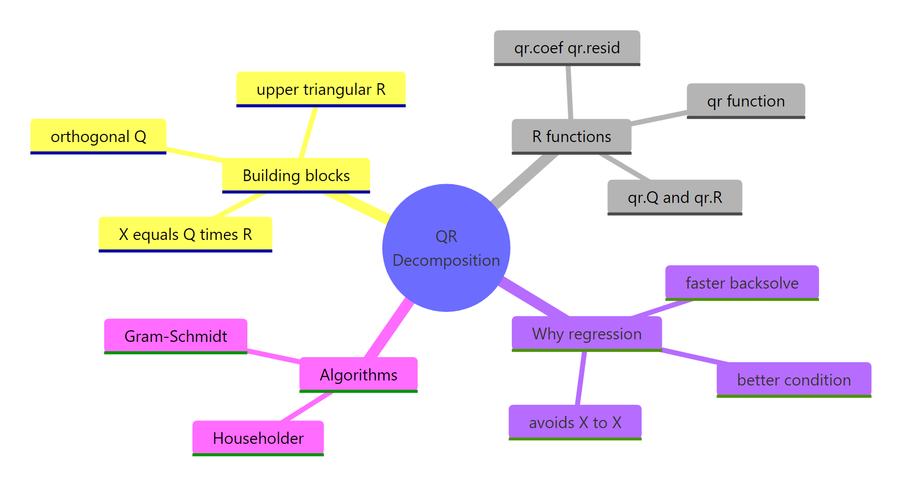
QR decomposition in R: building blocks, R functions, why regression uses it, and algorithms

Figure 3: Big-picture map of QR decomposition concepts, R functions, and algorithms.

Concept	What to remember	Function
Factorization	$X = QR$ with orthogonal $Q$ and upper triangular $R$	`qr()`, `qr.Q()`, `qr.R()`
Why for regression	Avoids squaring $\kappa(X)$ that $X^\top X$ would cause	`qr.coef()`, `qr.solve()`
Inside lm()	`fit$qr` is a stored `qr` object; helpers reuse it	`qr.fitted()`, `qr.resid()`
Algorithms	Householder is what base R uses; Gram-Schmidt is the textbook version	`qr()` (LINPACK / LAPACK)
Rank-deficient	`qr()$rank` and `qr()$pivot` reveal collinear columns	`tol =` argument

Key Insight

If you ever feel tempted to write solve(t(X) %*% X) %*% t(X) %*% y, write qr.solve(X, y) instead. The QR call is a one-liner, runs no slower, and avoids the conditioning trap that has bitten OLS implementations for half a century.

References

R Core Team , qr: The QR Decomposition of a Matrix. R help page. Link
Trefethen, L. N. & Bau, D. , Numerical Linear Algebra. SIAM (1997). Lectures 7-10 (Householder, QR, conditioning).
Wickham, H. , Advanced R, 2nd Edition. CRC Press (2019). Link
Larget, B. , The QR Decomposition and Regression, Statistics 496, UW-Madison. Link
Irizarry, R. , Genomics Class: The QR decomposition. Link
Strang, G. , Introduction to Linear Algebra, 5th Edition. Wellesley-Cambridge (2016). Chapter 4: Orthogonality.

Continue Learning

Solving Linear Systems in R: solve(), qr() & Least Squares Solutions , when to call solve() vs qr.solve() for square and overdetermined systems.
Projections & the Hat Matrix in R: OLS Geometry Explained Visually , how the hat matrix $H = X(X^\top X)^{-1} X^\top$ becomes a clean projection once you know QR.
Singular Value Decomposition in R: svd() & The Most Useful Matrix Operation , SVD generalises QR and handles rank-deficiency without pivoting.