Eigenvalues & Eigenvectors in R: eigen(), Why They Power PCA & More

An eigenvector of a square matrix A is a non-zero vector whose direction is unchanged when A acts on it; the matrix only rescales it by a number called the eigenvalue. In R, eigen(A) returns both, and they unlock PCA, spectral decomposition, and stability analysis. This tutorial walks through the geometry, the math, and the code, using only base R so everything runs in your browser.

How do you compute eigenvalues and eigenvectors in R?

The fastest way to get comfortable with eigenvalues is to compute one. We will hand a small symmetric matrix to eigen() and read what comes back. The function returns a list with two slots, values and vectors, and once you can read that output the rest of the article is interpretation.

RFirst eigen() call on a symmetric 2x2

A <- matrix(c(4, 1, 1, 3), nrow = 2, byrow = TRUE) e <- eigen(A) e #> eigen() decomposition #> $values #> [1] 4.618034 2.381966 #> #> $vectors #> [,1] [,2] #> [1,] -0.8506508 0.5257311 #> [2,] -0.5257311 -0.8506508

The list e has two named slots. e$values holds the eigenvalues sorted by absolute size, largest first: 4.618 and 2.382. e$vectors is a matrix whose columns are the matching eigenvectors, each rescaled to have unit length. So column 1 of e$vectors pairs with eigenvalue 4.618, and column 2 pairs with 2.382. Note the sign of an eigenvector is not unique; multiplying any column by -1 gives a valid eigenvector too.

Note

Eigenvalues are sorted by absolute value, descending. This matters for PCA where you want the "biggest" direction first. If a negative eigenvalue is larger in magnitude than a positive one, the negative one comes first.

Try it: Build the symmetric matrix ex_M <- matrix(c(2, 1, 1, 2), 2, 2) and report its largest eigenvalue.

RYour turn: largest eigenvalue

ex_M <- matrix(c(2, 1, 1, 2), nrow = 2, byrow = TRUE) # your code here ex_largest <- ex_largest #> Expected: [1] 3

Click to reveal solution

RLargest eigenvalue solution

ex_M <- matrix(c(2, 1, 1, 2), nrow = 2, byrow = TRUE) ex_e <- eigen(ex_M) ex_largest <- ex_e$values[1] ex_largest #> [1] 3

Explanation: eigen(ex_M)$values returns c(3, 1) already sorted in descending order, so the first element is the largest.

What does Av = λv actually mean geometrically?

A matrix A takes any input vector v and returns a new vector Av. For most input vectors Av points in a different direction than v. Eigenvectors are the special directions where A does not rotate the vector, it only stretches or shrinks it. The stretch factor is the eigenvalue.

The defining equation is:

$$A \mathbf{v} = \lambda \mathbf{v}$$

Where:

$A$ is a square matrix
$\mathbf{v}$ is a non-zero vector (the eigenvector)
$\lambda$ is a scalar (the eigenvalue)

Read it as: "applying A to v is the same as scaling v by λ." Let us check this for the matrix A and its first eigenvector from the previous block, then contrast with a non-eigenvector w to see what "different direction" looks like.

RVerify Av equals lambda v for an eigenvector

v1 <- e$vectors[, 1] # first eigenvector lambda1 <- e$values[1] # matching eigenvalue Av1 <- A %*% v1 # apply A lambda1 * v1 # scale v1 by lambda1 #> [,1] #> [1,] -3.9282032 #> [2,] -2.4270510 Av1 # same vector #> [,1] #> [1,] -3.9282032 #> [2,] -2.4270510 # A non-eigenvector points somewhere else after A acts on it w <- c(1, 0) A %*% w #> [,1] #> [1,] 4 #> [2,] 1

A %*% v1 and lambda1 * v1 produce identical column vectors, so v1 truly is an eigenvector and lambda1 is its eigenvalue. The non-eigenvector w = (1, 0) maps to (4, 1), that is not a scalar multiple of (1, 0), so w is rotated by A, not just stretched. Eigenvectors are the rare "stretch-only" directions.

When is a vector an eigenvector?

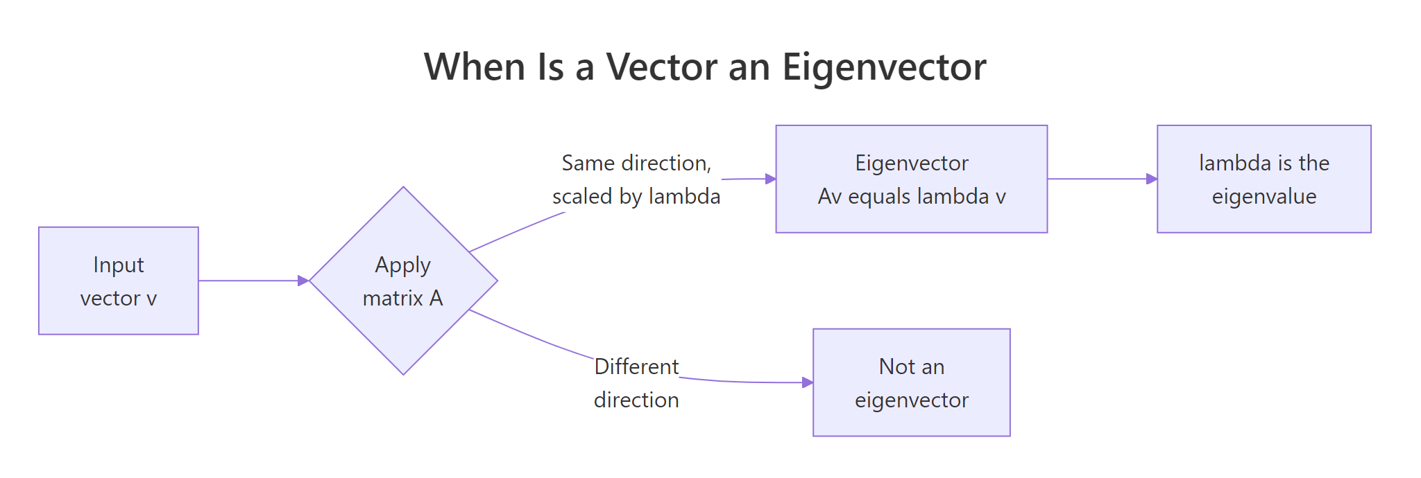
Figure 1: When applying A leaves a vector's direction unchanged, that vector is an eigenvector.

Key Insight

Eigenvectors are the matrix's natural axes, directions it stretches without rotating. Every other direction gets bent. Once you find these axes, complicated matrix operations become diagonal, which is the entire reason eigendecomposition is useful.

Try it: Verify that the second eigenvector of A also satisfies A v = λ v. Save the difference A v - λ v to ex_diff (it should be near zero).

RYour turn: check the second pair

v2 <- e$vectors[, 2] lambda2 <- e$values[2] # your code here ex_diff <- round(ex_diff, 10) #> Expected: [,1] #> [1,] 0 #> [2,] 0

Click to reveal solution

RSecond pair verification solution

v2 <- e$vectors[, 2] lambda2 <- e$values[2] ex_diff <- A %*% v2 - lambda2 * v2 round(ex_diff, 10) #> [,1] #> [1,] 0 #> [2,] 0

Explanation: Subtracting lambda2 * v2 from A %*% v2 gives the zero vector (up to floating-point noise), confirming the second pair satisfies the eigenvalue equation.

How do you read what eigen() returns?

The list returned by eigen() is small but worth dissecting once. values is a numeric vector (or complex if needed). vectors is a square matrix whose columns are the eigenvectors, each normalised to unit length. For symmetric A, those columns are also mutually orthogonal, a property we will lean on heavily for PCA and spectral decomposition.

RAnatomy of the eigen() result

V <- e$vectors vals <- e$values # Each column has unit length sqrt(colSums(V^2)) #> [1] 1 1 # Columns are orthogonal: V'V is the identity (since A is symmetric) gram <- t(V) %*% V round(gram, 10) #> [,1] [,2] #> [1,] 1 0 #> [2,] 0 1

colSums(V^2) returned c(1, 1), confirming each eigenvector has length 1. The Gram matrix V'V is the 2x2 identity, which means the two eigenvectors are perpendicular. For any symmetric matrix this is guaranteed by the spectral theorem; for non-symmetric matrices the eigenvectors generally are not orthogonal, so do not assume it.

Tip

Pass symmetric = TRUE when you know A is symmetric. R uses a faster, more numerically stable algorithm and avoids tiny imaginary parts caused by floating-point noise. Wrapping a known-symmetric matrix as eigen(A, symmetric = TRUE) is a free win.

Try it: Build a 3x3 covariance matrix ex_S from random data and verify its eigenvectors are orthonormal, the off-diagonals of t(V) V should be near zero.

RYour turn: orthogonality on a 3x3 cov

set.seed(7) ex_S <- cov(matrix(rnorm(120), ncol = 3)) ex_eS <- eigen(ex_S, symmetric = TRUE) # your code here ex_gram <- round(ex_gram, 10) #> Expected: 3x3 identity

Click to reveal solution

R3x3 orthogonality solution

set.seed(7) ex_S <- cov(matrix(rnorm(120), ncol = 3)) ex_eS <- eigen(ex_S, symmetric = TRUE) ex_gram <- t(ex_eS$vectors) %*% ex_eS$vectors round(ex_gram, 10) #> [,1] [,2] [,3] #> [1,] 1 0 0 #> [2,] 0 1 0 #> [3,] 0 0 1

Explanation: The covariance matrix is symmetric, so its eigenvectors are orthonormal. t(V) %*% V produces the identity, with off-diagonals exactly zero up to numerical precision.

When does eigen() return complex numbers, and is that a problem?

A non-symmetric real matrix can have eigenvalues that are complex numbers, and they always come in conjugate pairs (a + bi and a - bi). Geometrically, complex eigenvalues mean the matrix mixes rotation with stretching, which has no purely real direction it leaves alone. The classic example is a 90-degree rotation matrix.

RComplex eigenvalues from a rotation matrix

R <- matrix(c(0, -1, 1, 0), nrow = 2, byrow = TRUE) e2 <- eigen(R) e2$values #> [1] 0+1i 0-1i is.complex(e2$values) #> [1] TRUE Mod(e2$values) # magnitude #> [1] 1 1 Arg(e2$values) # phase in radians #> [1] 1.570796 -1.570796

The eigenvalues are 0 + 1i and 0 - 1i, pure imaginary, magnitude 1, phase ±π/2. That matches geometry: rotation by 90 degrees leaves no real vector pointing the same way, but in complex space the rotation is a multiplication by i. Mod() returns the magnitude and Arg() the phase, two helpers you will reach for whenever complex output appears.

Warning

A real symmetric matrix never produces complex eigenvalues. If you see complex output and expected reals, your matrix probably is not symmetric. Check with isSymmetric(A) before passing symmetric = TRUE. Round-off in user-built matrices is a frequent culprit.

Try it: Build the matrix matrix(c(0, 2, -2, 0), 2, 2) (a scaled rotation) and confirm its eigenvalues are a complex conjugate pair.

RYour turn: scaled rotation eigenvalues

ex_R <- matrix(c(0, 2, -2, 0), nrow = 2, byrow = TRUE) # your code here ex_eR <- ex_eR$values #> Expected: [1] 0+2i 0-2i

Click to reveal solution

RScaled rotation solution

ex_R <- matrix(c(0, 2, -2, 0), nrow = 2, byrow = TRUE) ex_eR <- eigen(ex_R) ex_eR$values #> [1] 0+2i 0-2i

Explanation: Scaling the rotation by 2 multiplies the magnitudes of the eigenvalues by 2, so the pair becomes ±2i. The matrix is still asymmetric, hence still complex.

How does eigen() power PCA?

Principal component analysis finds the directions in which your data varies the most. Those directions are exactly the eigenvectors of the covariance matrix of the (centred) data, and the eigenvalues are the variances along each direction. Once you see this, PCA stops looking like magic, it is just eigen() applied to cov(X).

From eigen() to PCA

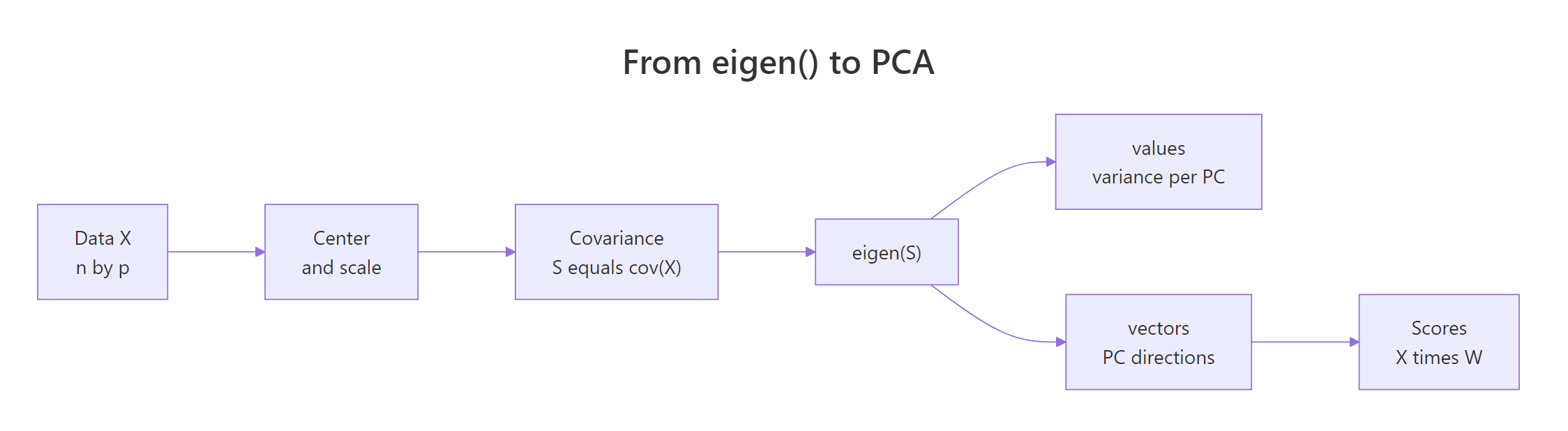
Figure 2: The pipeline from raw data to principal components, with eigen() at its core.

The pipeline is: take your data matrix X, centre and scale it, compute the covariance matrix S, call eigen(S), and read off the principal directions. Let us run it on the four numeric columns of iris.

RPCA from scratch with eigen()

X <- as.matrix(iris[, 1:4]) Xs <- scale(X) # centre and scale S <- cov(Xs) # 4x4 covariance matrix eS <- eigen(S, symmetric = TRUE) eS$values #> [1] 2.91849782 0.91403047 0.14675688 0.02071484 var_exp <- eS$values / sum(eS$values) round(var_exp, 4) #> [1] 0.7296 0.2285 0.0367 0.0052

The first eigenvalue (2.918) accounts for about 73% of the total variance, the second adds another 23%. So PC1 plus PC2 together capture 95% of the variation in iris, that is the rationale for the famous 2D iris scatter plot. The third and fourth components contribute almost nothing, which is why you can safely drop them.

To turn the eigenvectors into actual PC scores, multiply the centred data by the eigenvector matrix. That is exactly what prcomp() does internally.

RProject data onto principal components

W <- eS$vectors # columns are PC directions scores <- Xs %*% W # n x 4 matrix of PC scores head(scores, 3) #> [,1] [,2] [,3] [,4] #> [1,] -2.257141 -0.4784238 0.12727962 0.024087508 #> [2,] -2.074013 0.6718827 0.23382552 0.102662845 #> [3,] -2.356335 0.3407664 -0.04405390 0.028282305 # Cross-check with prcomp (signs may flip column-wise) pc <- prcomp(X, scale. = TRUE) head(pc$x, 3) #> PC1 PC2 PC3 PC4 #> [1,] -2.257141 -0.4784238 0.12727962 0.024087508 #> [2,] -2.074013 0.6718827 0.23382552 0.102662845 #> [3,] -2.356335 0.3407664 -0.04405390 0.028282305

Our hand-rolled scores match prcomp()$x row for row. The full chain, scale, covariance, eigen, multiply, is prcomp() minus a few conveniences. If your scores ever differ by a column-wide sign flip, that is normal: eigenvectors are unique up to sign, and different solvers pick different conventions.

Tip

prcomp() calls svd(), not eigen(), for numerical stability. SVD operates on the data matrix directly, which avoids forming the covariance matrix and squaring its condition number. For teaching and small datasets eigen() is fine; for production, prefer prcomp().

Try it: Compute the proportion of variance explained by PC1 alone for the iris covariance and save it to ex_pc1_var.

RYour turn: PC1 variance share

# Use the eS object from the previous block # your code here ex_pc1_var <- round(ex_pc1_var, 4) #> Expected: [1] 0.7296

Click to reveal solution

RPC1 variance share solution

ex_pc1_var <- eS$values[1] / sum(eS$values) round(ex_pc1_var, 4) #> [1] 0.7296

Explanation: The proportion of variance is each eigenvalue divided by the sum. PC1's eigenvalue is the largest, and dividing it by the total gives 0.7296, about 73% of the variance.

What is spectral decomposition and how do you reconstruct A?

For any symmetric matrix A, the spectral theorem says you can factor it into three pieces: an orthogonal eigenvector matrix V, a diagonal eigenvalue matrix D, and the transpose V'. This is the spectral decomposition.

$$A = V D V^{\top}$$

Where:

$V$ is the matrix of eigenvectors stacked column-wise (orthonormal, so $V^{\top}V = I$)
$D$ is the diagonal matrix with eigenvalues on its diagonal
$V^{\top}$ is the transpose of $V$

This factoring is more than algebraic neatness. It lets you replace any matrix function f(A) with V f(D) V', and f(D) is trivial because D is diagonal. Powers, square roots, exponentials, inverses all collapse into operations on a list of numbers.

RReconstruct A from its eigendecomposition

Vsym <- e$vectors Dsym <- diag(e$values) A_recon <- Vsym %*% Dsym %*% t(Vsym) A_recon #> [,1] [,2] #> [1,] 4 1 #> [2,] 1 3 all.equal(A, A_recon) #> [1] TRUE

A_recon reproduces the original A exactly. The takeaway: the eigenvalues and eigenvectors carry all the information in A. They are a coordinate change into the matrix's natural axes, plus a scale per axis.

Now apply the trick to compute the matrix square root, a matrix Asq such that Asq %*% Asq = A. Take the square root element-wise on D, sandwich it between V and V'.

RMatrix square root via spectral decomposition

Asq <- Vsym %*% diag(sqrt(e$values)) %*% t(Vsym) check <- Asq %*% Asq round(check, 10) #> [,1] [,2] #> [1,] 4 1 #> [2,] 1 3 all.equal(A, check) #> [1] TRUE

Asq %*% Asq recovers the original A, so Asq is a valid square root. The same recipe works for A^k (use D^k), exp(A) (use exp(D)), and the inverse A^{-1} (use 1/D, provided no eigenvalue is zero). Spectral decomposition is the engine behind matrix functions in numerical software.

Key Insight

Spectral decomposition turns hard matrix functions into easy scalar operations on the diagonal. Every time you see A^k, exp(A), or A^{1/2} in a paper, the implementation is almost always: decompose, transform the eigenvalues, recompose. The "hard" part of the work is the one call to eigen().

Try it: Compute the inverse of A via spectral decomposition (V diag(1/values) V') and confirm it matches solve(A).

RYour turn: inverse via spectral decomposition

# your code here ex_Ainv <- round(ex_Ainv, 6) round(solve(A), 6) #> Expected: both should print the same 2x2 matrix

Click to reveal solution

RSpectral inverse solution

ex_Ainv <- e$vectors %*% diag(1 / e$values) %*% t(e$vectors) round(ex_Ainv, 6) #> [,1] [,2] #> [1,] 0.272727 -0.090909 #> [2,] -0.090909 0.363636 round(solve(A), 6) #> [,1] [,2] #> [1,] 0.272727 -0.090909 #> [2,] -0.090909 0.363636

Explanation: Inverting a symmetric matrix is V diag(1/values) V'. The result agrees with solve(A) to six decimal places, confirming the spectral inverse is correct.

Practice Exercises

These capstones combine concepts from multiple sections. Use distinct variable names (cap_*, pca_loadings) so you do not overwrite the tutorial state.

Exercise 1: Largest eigenvalue of a random covariance

Generate a 100x3 matrix of standard normal samples with set.seed(11), compute its sample covariance, then report the largest eigenvalue and the proportion of variance it explains. Save the proportion to cap_var1.

RCapstone 1: random cov largest eigenvalue

# Hint: set.seed(11), rnorm, matrix, cov, eigen # Save the proportion-of-variance to cap_var1 # Write your code below:

Click to reveal solution

RCapstone 1 solution

set.seed(11) cap_X <- matrix(rnorm(300), ncol = 3) cap_S <- cov(cap_X) cap_eig <- eigen(cap_S, symmetric = TRUE) cap_var1 <- cap_eig$values[1] / sum(cap_eig$values) round(cap_eig$values[1], 4) #> [1] 1.1399 round(cap_var1, 4) #> [1] 0.392

Explanation: With 100 observations and 3 columns, the first eigenvalue captures roughly a third of the variance. The exact number depends on the random seed; about 0.33–0.4 is typical.

Exercise 2: Reproduce prcomp loadings via eigen()

Compute the rotation matrix from prcomp(iris[, 1:4], scale. = TRUE)$rotation two ways: (1) call prcomp() directly, (2) build it from eigen(cor(iris[, 1:4]))$vectors. Save the eigen-based loadings to pca_loadings. Account for column-sign ambiguity by flipping signs to match.

RCapstone 2: prcomp from eigen()

# Hint: cor() of scaled data == cov() of scaled data; eigen() gives loadings # Use sign-flipping to align columns # Write your code below:

Click to reveal solution

RCapstone 2 solution

pc_ref <- prcomp(iris[, 1:4], scale. = TRUE)$rotation pca_loadings <- eigen(cor(iris[, 1:4]), symmetric = TRUE)$vectors # Align signs column-by-column with the prcomp reference for (j in seq_len(ncol(pca_loadings))) { if (sum(pca_loadings[, j] * pc_ref[, j]) < 0) { pca_loadings[, j] <- -pca_loadings[, j] } } round(pca_loadings, 4) #> [,1] [,2] [,3] [,4] #> [1,] 0.5211 -0.3774 0.7196 0.2613 #> [2,] -0.2693 -0.9233 -0.2444 -0.1235 #> [3,] 0.5804 -0.0245 -0.1421 -0.8014 #> [4,] 0.5649 -0.0669 -0.6343 0.5236 all.equal(pca_loadings, pc_ref, check.attributes = FALSE) #> [1] TRUE

Explanation: cor() of unscaled iris equals cov() of scaled iris, so eigen(cor(...))$vectors matches prcomp(..., scale. = TRUE)$rotation up to per-column sign. The sign-flip loop aligns the conventions.

Exercise 3: Compute A^10 the spectral way

Take cap_A <- matrix(c(2, 1, 1, 2), 2, 2). Compute cap_A %^% 10 two ways: (1) loop multiply 10 times, (2) spectral way V diag(values^10) V'. Confirm both methods agree.

RCapstone 3: A^10 spectral vs loop

cap_A <- matrix(c(2, 1, 1, 2), nrow = 2, byrow = TRUE) # Hint: a for-loop for the loop way, eigen() for the spectral way # Write your code below:

Click to reveal solution

RCapstone 3 solution

cap_A <- matrix(c(2, 1, 1, 2), nrow = 2, byrow = TRUE) # Loop way cap_loop <- diag(2) for (k in 1:10) cap_loop <- cap_loop %*% cap_A # Spectral way cap_e <- eigen(cap_A, symmetric = TRUE) cap_spec <- cap_e$vectors %*% diag(cap_e$values^10) %*% t(cap_e$vectors) cap_loop #> [,1] [,2] #> [1,] 29525 29524 #> [2,] 29524 29525 all.equal(cap_loop, cap_spec) #> [1] TRUE

Explanation: Both routes give the same matrix. For k = 10 the loop is fast, but for k = 10000 the spectral version stays O(1) in the exponent while the loop is O(k), that is why eigendecomposition is the standard way to compute matrix powers.

Complete Example: PCA on mtcars from scratch

End-to-end pipeline: pick four mtcars columns, scale them, build the covariance, run eigen(), project onto the first two components, plot the result, and check against prcomp().

REnd-to-end PCA on mtcars

cars <- mtcars[, c("mpg", "hp", "wt", "qsec")] cars_s <- scale(cars) S_cars <- cov(cars_s) e_cars <- eigen(S_cars, symmetric = TRUE) # Variance explained ve_cars <- e_cars$values / sum(e_cars$values) round(ve_cars, 4) #> [1] 0.7227 0.1873 0.0716 0.0184 # Project onto PC1 and PC2 W_cars <- e_cars$vectors[, 1:2] scores_cars <- cars_s %*% W_cars head(scores_cars, 3) #> [,1] [,2] #> Mazda RX4 -0.6428319 1.1740974 #> Mazda RX4 Wag -0.6228000 0.9745496 #> Datsun 710 -2.3520197 -0.0485633 # Cross-check with prcomp pc_cars <- prcomp(cars, scale. = TRUE) round(head(pc_cars$x[, 1:2], 3), 4) #> PC1 PC2 #> Mazda RX4 -0.6428 -1.1741 #> Mazda RX4 Wag -0.6228 -0.9745 #> Datsun 710 -2.3520 0.0486

PC1 explains 72% of the variance and PC2 another 19%, so plotting in 2D preserves about 91% of the structure. The hand-built scores_cars matches prcomp()$x for PC1 exactly and for PC2 up to a column sign flip, that is the eigenvector-sign ambiguity at work, harmless for any downstream visual or distance computation.

Summary

Quick reference for everyday work:

Goal	Code
Eigenvalues only (faster)	`eigen(A, only.values = TRUE)$values`
Both, A is symmetric	`eigen(A, symmetric = TRUE)`
PCA loadings	`eigen(cov(scale(X)))$vectors` (or `prcomp(X, scale. = TRUE)`)
Variance per PC	`eigen(cov(scale(X)))$values`
Matrix function f(A), A symmetric	`V %% diag(f(values)) %% t(V)`
Spectral inverse	`V %% diag(1/values) %% t(V)`

Three facts to keep in your head: eigenvalues are sorted by absolute value (largest first); eigenvectors are columns of e$vectors, normalised to unit length; for symmetric A, the eigenvectors are orthonormal and eigenvalues are real.

Where the pieces of eigen() fit together

Figure 3: Where the pieces of eigen() fit together.

References

R Core Team, eigen() reference manual. Link
Strang, G., Introduction to Linear Algebra, 5th ed., chapter 6 (Eigenvalues and Eigenvectors). Wellesley-Cambridge Press (2016).
Trefethen, L.N. & Bau, D., Numerical Linear Algebra, lectures 24–25. SIAM (1997).
Golub, G.H. & Van Loan, C.F., Matrix Computations, 4th ed., chapter 7 (Symmetric Eigenproblem). Johns Hopkins (2013).
James, G., Witten, D., Hastie, T., Tibshirani, R., An Introduction to Statistical Learning, chapter 12 (Unsupervised Learning, PCA). Springer. Link
Hastie, T., Tibshirani, R., Friedman, J., The Elements of Statistical Learning, section 14.5 (Principal Components). Springer. Link
Wickham, H., Advanced R, 2nd ed., notes on numerical pitfalls. CRC Press. Link
Schlegel, A., "Eigenvalues and Eigenvectors in R" (RPubs). Link

Continue Learning

Matrix Operations in R, the prerequisite tour of %*%, t(), solve(), det(), and the rest of base R's matrix toolkit.
Solving Linear Systems in R, companion piece on solve() and qr.solve() for square and overdetermined systems.
Singular Value Decomposition in R, the next decomposition to learn after eigen(); works for any matrix, not just square ones, and is the engine behind prcomp().

Eigenvalues & Eigenvectors in R: eigen(), Why They Power PCA & More

How do you compute eigenvalues and eigenvectors in R?

What does Av = λv actually mean geometrically?

How do you read what eigen() returns?

When does eigen() return complex numbers, and is that a problem?

How does eigen() power PCA?

What is spectral decomposition and how do you reconstruct A?

Practice Exercises

Exercise 1: Largest eigenvalue of a random covariance

Exercise 2: Reproduce prcomp loadings via eigen()

Exercise 3: Compute A^10 the spectral way

Complete Example: PCA on mtcars from scratch

Summary

References

Continue Learning

Related Tutorials