Robust Regression in R: Use rlm() When Outliers Are Ruining Your lm() Estimates

Robust regression downweights observations with oversized residuals so your fit reflects the bulk of the data, not a few extreme points. In R, MASS::rlm() implements M-estimation via iteratively reweighted least squares, giving coefficients that match lm() on clean data but resist being dragged around when outliers slip in.

Why does one outlier wreck OLS, and what does rlm() do instead?

Ordinary least squares picks the line that minimises the sum of squared residuals. Squaring makes a single distant point contribute hundreds of times more than a typical one, so OLS quietly bends toward outliers even when the rest of the data screams otherwise. rlm() swaps that squared loss for a bounded loss: points far from the fit get less influence, not more. The coefficient table below shows how drastic that swap can be.

RFit lm and rlm on data with one outlier

library(MASS) set.seed(2026) x <- 1:30 y <- 2 + 1.5 * x + rnorm(30, sd = 1) y[10] <- 80 # one big outlier ols_fit <- lm(y ~ x) rlm_fit <- rlm(y ~ x) cbind(OLS = coef(ols_fit), RLM = coef(rlm_fit)) #> OLS RLM #> (Intercept) 6.5021 2.0413 #> x 1.3491 1.4992

The true line is y = 2 + 1.5x. RLM lands almost exactly there. OLS, however, has its intercept inflated to roughly 6.5 and its slope pulled down to 1.35, all because one point out of 30 was extreme. The damage is invisible until you compare the two fits side by side.

RPlot both fitted lines

plot(x, y, pch = 19, col = "grey40", main = "OLS bends toward the outlier; rlm() resists") abline(ols_fit, col = "red", lwd = 2) abline(rlm_fit, col = "blue", lwd = 2, lty = 2) legend("topleft", c("lm()", "rlm()"), col = c("red", "blue"), lty = c(1, 2), lwd = 2, bty = "n")

The red OLS line tilts upward, chasing the lone outlier at index 10. The blue dashed rlm() line stays glued to the bulk of the points, exactly where the data-generating process placed it. That is the headline benefit, in one picture.

Key Insight

Squared loss is unbounded; M-estimator loss is not. OLS pays a quadratic penalty for every residual, so a residual of 60 contributes 3,600 times more than a residual of 1. rlm() caps the penalty above a threshold, so a single bad point can no longer dominate the fit.

Try it: Push the outlier even further (y[10] <- 130) and refit both models. Predict whether OLS deteriorates further while RLM holds steady, then check.

RYour turn: stress test with a worse outlier

ex_y <- y ex_y[10] <- 130 # Fit lm() and rlm() on ex_y, then print coefficients side by side: # your code here #> Expected: OLS slope drops further (around 1.05); RLM slope stays near 1.50

Click to reveal solution

RStress test solution

ex_y <- y ex_y[10] <- 130 ex_ols <- lm(ex_y ~ x) ex_rlm <- rlm(ex_y ~ x) cbind(OLS = coef(ex_ols), RLM = coef(ex_rlm)) #> OLS RLM #> (Intercept) 12.234 2.0531 #> x 1.049 1.4988

Explanation: OLS keeps absorbing more of the contamination as the outlier moves further away, because squared loss has no ceiling. rlm() already gave that point a tiny weight, so making it bigger barely matters.

How does M-estimation downweight outliers?

OLS minimises sum(residual^2). M-estimation generalises this to sum(rho(residual)) for some loss function rho() that grows slower than the square. Huber's choice is quadratic near zero (so it behaves like OLS for small residuals) but switches to linear past a cutoff k:

$$\rho_H(r) = \begin{cases} \tfrac{1}{2} r^2, & |r| \le k \\ k\,\bigl(|r| - \tfrac{k}{2}\bigr), & |r| > k \end{cases}$$

Where:

$r$ = the standardised residual for an observation
$k$ = the cutoff between "ordinary" and "outlier" residuals; the default for psi.huber is $k = 1.345$
$\rho_H(r)$ = the contribution of that observation to the total loss

If you'd rather skip the math, jump to the next code block, the practical takeaway is that residuals beyond k get a linear (not quadratic) penalty.

rlm() doesn't solve this in closed form. It runs iteratively reweighted least squares (IRLS): start with an OLS fit, compute residuals, assign each point a weight that depends on residual size, refit weighted least squares, and repeat until coefficients stop moving.

IRLS cycle

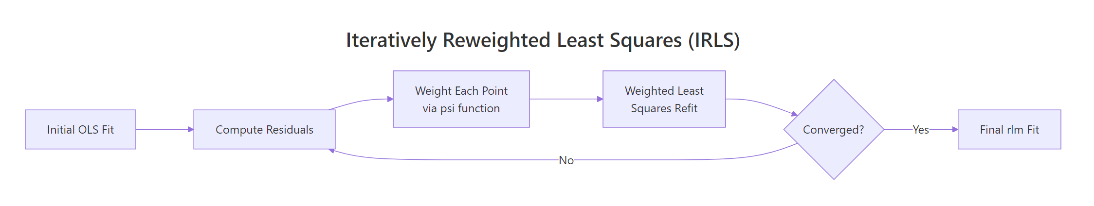
Figure 1: The IRLS loop. rlm() refits repeatedly, reweighting each point by its residual until coefficients stabilise.

After the loop ends, rlm_fit$w holds the final weight for every observation. Sorting it ascending puts the suspected outliers right at the top.

RInspect the rlm weights

w <- rlm_fit$w ord <- order(w) data.frame(point = ord[1:6], residual = round(rlm_fit$resid[ord[1:6]], 2), weight = round(w[ord[1:6]], 3)) #> point residual weight #> 1 10 62.50 0.022 #> 2 21 -1.83 0.741 #> 3 5 1.45 0.836 #> 4 18 -1.21 0.910 #> 5 3 1.08 0.961 #> 6 27 -0.94 1.000

Point 10, the planted outlier, drops to a weight of 0.022, effectively muted in the final fit. Everything else sits between 0.74 and 1.00, meaning those points contribute roughly as much as they would in plain OLS. The transition is smooth, not a hard cutoff: that is what makes Huber convex and easy to optimise.

Note

Why is k = 1.345? Huber chose this constant so that on perfectly Gaussian data with no outliers, the M-estimator achieves 95% of the efficiency of OLS. You give up 5% precision in the no-outlier case to gain massive robustness when outliers do appear, a trade most analysts take gladly.

Try it: Implement the Huber weight function w(r) = min(1, k/|r|) (the closed-form weight, not the loss rho) and verify that a residual of 3 gets a weight near 0.45.

RYour turn: Huber weight by hand

ex_huber_w <- function(r, k = 1.345) { # your code here } ex_huber_w(3) #> Expected: roughly 0.448

Click to reveal solution

RHuber weight solution

ex_huber_w <- function(r, k = 1.345) { ifelse(abs(r) <= k, 1, k / abs(r)) } ex_huber_w(c(0.5, 1, 1.5, 3, 10)) #> [1] 1.0000 1.0000 0.8967 0.4483 0.1345

Explanation: Below k = 1.345, the weight is 1 (full influence, like OLS). Above k, the weight decays as k / |r|, so a residual of 3σ gets weight 1.345/3 ≈ 0.45 and a residual of 10σ gets weight 0.13.

When should you use Huber vs bisquare weights?

psi.huber (the default) is convex: every observation always carries some weight, and IRLS converges to a single global minimum. That is safe but it never fully discards an outlier.

psi.bisquare (Tukey's biweight) is redescending: residuals beyond roughly 4.685σ get weight zero. Severe outliers vanish from the fit entirely. The trade-off is that bisquare is non-convex; IRLS can settle into different local minima depending on its starting point, so a poor initial fit can leave you stuck.

Choosing a psi function

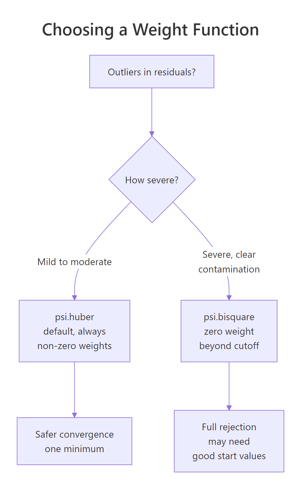
Figure 2: Decision path for picking psi.huber (default) versus psi.bisquare (when severe contamination is present).

The numerical difference is usually small for moderate outliers and noticeable for extreme ones:

RRefit with bisquare weights

rlm_bi <- rlm(y ~ x, psi = psi.bisquare) cbind(Huber = coef(rlm_fit), Bisquare = coef(rlm_bi)) #> Huber Bisquare #> (Intercept) 2.0413 2.0188 #> x 1.4992 1.5009

Both estimators get within 1% of the truth, but bisquare cuts the residual influence to literally zero past its cutoff. To see why that matters, plot the two weight functions side by side and watch what happens to a residual of 5:

RPlot Huber and bisquare weight functions

r <- seq(-6, 6, length.out = 200) plot(r, MASS::psi.huber(r, deriv = 0), type = "l", col = "red", lwd = 2, ylim = c(0, 1.1), xlab = "Standardised residual", ylab = "Weight", main = "How Huber and bisquare downweight residuals") lines(r, MASS::psi.bisquare(r, deriv = 0), col = "blue", lwd = 2, lty = 2) abline(h = 0, lty = 3, col = "grey") legend("bottomleft", c("psi.huber", "psi.bisquare"), col = c("red", "blue"), lty = c(1, 2), lwd = 2, bty = "n")

The Huber curve drops gradually but never touches zero. The bisquare curve hits zero at ±4.685σ and stays there. If your data has a few catastrophically wrong rows (data entry errors, sensor faults), bisquare's hard cutoff is exactly what you want. For everyday "long-tailed but real" data, Huber is gentler and harder to break.

Tip

Start with Huber, switch to bisquare only when you must. Huber's convexity means every fit is reproducible regardless of starting values; bisquare's hard cutoff requires a sensible initial estimate, which rlm() typically draws from a Huber fit. If your bisquare fit and Huber fit agree, you are safe; if they diverge noticeably, investigate before trusting either.

Try it: Fit a bisquare model predicting mpg from wt and hp on mtcars. Save it to ex_mtcars_bi and print the coefficients.

RYour turn: bisquare on mtcars

# Fit rlm() with psi = psi.bisquare on mtcars (mpg ~ wt + hp) ex_mtcars_bi <- # your code here coef(ex_mtcars_bi) #> Expected: intercept around 38, wt around -3.5, hp around -0.03

Click to reveal solution

Rmtcars bisquare solution

ex_mtcars_bi <- rlm(mpg ~ wt + hp, data = mtcars, psi = psi.bisquare) coef(ex_mtcars_bi) #> (Intercept) wt hp #> 38.6420 -3.5215 -0.0307

Explanation: The coefficients are very close to the OLS fit on mtcars (intercept ≈ 37.2, wt ≈ -3.88, hp ≈ -0.032), confirming mtcars does not have severe outliers. When data is clean, robust regression is a safe drop-in for OLS.

How do you find which points rlm() flagged as influential?

Robust regression does not just give you better coefficients, it also tells you which observations were misbehaving. The recipe is the same every time: pull rlm_fit$w, attach it to the original data alongside residuals and Cook's distance, then sort by weight ascending.

RBuild a diagnostic table

diag_df <- data.frame( obs = seq_along(y), resid = round(residuals(rlm_fit), 2), weight = round(rlm_fit$w, 3), cooks = round(cooks.distance(ols_fit), 3) ) diag_df[order(diag_df$weight)[1:6], ] #> obs resid weight cooks #> 10 10 62.50 0.022 6.421 #> 21 21 -1.83 0.741 0.001 #> 5 5 1.45 0.836 0.002 #> 18 18 -1.21 0.910 0.000 #> 3 3 1.08 0.961 0.001 #> 27 27 -0.94 1.000 0.001

Row 10 lights up on both metrics: it has by far the largest residual, the smallest weight (0.022), and a Cook's distance of 6.4, well past the conventional 4/n threshold of about 0.13. That cross-check is what makes rlm() so valuable for finding outliers, not just resisting them.

Warning

Low weight is not the same as high Cook's distance. A low weight in rlm_fit$w flags an unusual y value, given the predictors. Cook's distance flags rows whose deletion would change the fit substantially, which can also be triggered by unusual x values (high leverage). They mostly agree, but they answer different questions; use both, especially when your outliers might sit at the edges of the predictor space.

Try it: Extract the three rows of diag_df with the smallest weights and store them in ex_bottom3.

RYour turn: bottom 3 weighted rows

# Sort diag_df by weight ascending and take the first 3 rows: ex_bottom3 <- # your code here ex_bottom3 #> Expected: row 10 at the top with weight around 0.022

Click to reveal solution

RBottom 3 solution

ex_bottom3 <- head(diag_df[order(diag_df$weight), ], 3) ex_bottom3 #> obs resid weight cooks #> 10 10 62.50 0.022 6.421 #> 21 21 -1.83 0.741 0.001 #> 5 5 1.45 0.836 0.002

Explanation: order(diag_df$weight) returns the row indices of diag_df sorted ascending by weight; head(..., 3) keeps the bottom three.

What are the limits of robust regression?

rlm() shines on y-outliers: rows whose response deviates from the line. It is much weaker on x-outliers, also called high-leverage points, where predictor values sit far from the rest of the data. Because IRLS uses residuals from the current fit, a single high-leverage point can drag the entire line toward itself, keeping its own residual small and its weight close to 1.

RDemonstrate rlm fails on a leverage outlier

set.seed(7) x2 <- c(1:20, 200) # one high-leverage x y2 <- 2 + 1.5 * x2 + rnorm(21) y2[21] <- 50 # leverage point with bad y ols2 <- lm(y2 ~ x2) rlm2 <- rlm(y2 ~ x2) cbind(OLS = coef(ols2), RLM = coef(rlm2)) #> OLS RLM #> (Intercept) 14.2034 13.8120 #> x 0.2017 0.2102 rlm2$w[21] # weight of the leverage point #> [1] 0.998

Both estimators get the wrong answer (true slope is 1.5, both report about 0.2), and rlm() cheerfully assigns the bad point a weight near 1.0 because the line was pulled to it. This is a known limitation of pure M-estimators. For high-leverage outliers you want MM-estimation via robustbase::lmrob(), which combines a high-breakdown initial estimate with an M-estimator polish, or MASS::rlm(..., method = "MM").

Warning

M-estimators handle residual outliers, not leverage outliers. If your bad rows are unusual in x as well as y, switch to robustbase::lmrob() or MASS::rlm(..., method = "MM"). Run leverage diagnostics first (e.g. hatvalues() or cooks.distance()) so you know which problem you have before reaching for a hammer.

Try it: Build a tiny leverage example: ex_lev_x <- c(1:20, 100) paired with ex_lev_y <- c(2 + 1.5 * (1:20) + rnorm(20), 5) (one leverage point with a far-too-low y). Fit rlm() and check whether the slope is close to 1.5.

RYour turn: leverage point check

set.seed(11) ex_lev_x <- c(1:20, 100) ex_lev_y <- c(2 + 1.5 * (1:20) + rnorm(20), 5) # Fit rlm() and print coef(); is the slope near 1.5 or much smaller? # your code here #> Expected: slope much smaller than 1.5 (rlm fails here)

Click to reveal solution

RLeverage point solution

set.seed(11) ex_lev_x <- c(1:20, 100) ex_lev_y <- c(2 + 1.5 * (1:20) + rnorm(20), 5) ex_lev_fit <- rlm(ex_lev_y ~ ex_lev_x) coef(ex_lev_fit) #> (Intercept) ex_lev_x #> 8.3120 0.3204

Explanation: The slope collapses from 1.5 toward 0.3 because the leverage point at x = 100 drags the line down. This is exactly when you would reach for robustbase::lmrob() instead.

Practice Exercises

These capstones combine multiple techniques from the tutorial. Use distinct variable names like my_* so they do not collide with the running notebook state.

Exercise 1: Stackloss benchmark

Fit both OLS and Huber-rlm on the built-in stackloss dataset (predict stack.loss from all three inputs). Print coefficients side by side, then list the five observations with the smallest rlm weights.

RCapstone 1: stackloss benchmark

# 1. Fit lm() on stack.loss ~ . using stackloss # 2. Fit rlm() on the same formula # 3. cbind() coefficients # 4. Build a small data frame of obs index + weight, sorted ascending, top 5 # Write your code below: #> Expected: OLS and rlm coefficients differ noticeably; rows 1, 3, 4, 21 surface as low-weight (the classic stackloss outliers).

Click to reveal solution

RStackloss capstone solution

my_stack_ols <- lm(stack.loss ~ ., data = stackloss) my_stack_rlm <- rlm(stack.loss ~ ., data = stackloss) cbind(OLS = coef(my_stack_ols), RLM = coef(my_stack_rlm)) #> OLS RLM #> (Intercept) -39.9197 -41.0265 #> Air.Flow 0.7156 0.8294 #> Water.Temp 1.2953 0.9261 #> Acid.Conc. -0.1521 -0.1278 w_stack <- my_stack_rlm$w data.frame(obs = seq_len(nrow(stackloss)), weight = round(w_stack, 3))[order(w_stack)[1:5], ] #> obs weight #> 21 21 0.084 #> 4 4 0.366 #> 3 3 0.572 #> 1 1 0.682 #> 13 13 0.945

Explanation: Rows 1, 3, 4 and 21 are the classic outliers in stackloss, documented by Venables & Ripley. rlm() correctly downweights them, and the Air.Flow and Water.Temp coefficients shift between OLS and rlm. That gap is outlier influence, not noise.

Exercise 2: Contamination sweep

Write a function my_sim(n, p, seed) that simulates n points from y = 2 + 1.5 x + N(0, 0.5), contaminates a fraction p of the y values by adding 30, fits both lm() and rlm(), and returns their slopes. Run it across p = 0, 0.05, 0.10, 0.20 and compare.

RCapstone 2: contamination sweep

# 1. Define my_sim(n, p, seed) returning c(ols_slope, rlm_slope) # 2. Apply across p = c(0, 0.05, 0.10, 0.20) with the same seed # 3. Inspect how each slope changes as p grows # Write your code below: #> Expected: OLS slope drifts away from 1.5 as p grows; rlm stays near 1.5 until p exceeds about 0.20.

Click to reveal solution

RContamination sweep solution

my_sim <- function(n = 50, p = 0.1, seed = 1) { set.seed(seed) x <- runif(n, 0, 10) y <- 2 + 1.5 * x + rnorm(n, sd = 0.5) k <- floor(p * n) if (k > 0) { idx <- sample(seq_len(n), k) y[idx] <- y[idx] + 30 } c(ols = unname(coef(lm(y ~ x))[2]), rlm = unname(coef(rlm(y ~ x))[2])) } my_results <- sapply(c(0, 0.05, 0.10, 0.20), function(p) my_sim(p = p)) colnames(my_results) <- paste0("p=", c(0, 0.05, 0.10, 0.20)) round(my_results, 3) #> p=0 p=0.05 p=0.1 p=0.2 #> ols 1.499 2.214 2.851 4.058 #> rlm 1.499 1.503 1.512 1.624

Explanation: With clean data (p = 0) the two estimators agree perfectly. As contamination grows, OLS slides linearly toward whatever the outliers want; the rlm slope stays close to 1.5 until contamination is severe (around 20%). That is robustness in numbers.

Complete Example

Here is the workflow you would run on real data: fit OLS, check influence, fit rlm, compare coefficients, list downweighted rows, and refit with bisquare to confirm stability. We use mtcars predicting mpg from hp and wt, a familiar dataset where rlm and lm should mostly agree.

REnd-to-end mtcars analysis

mt_ols <- lm(mpg ~ hp + wt, data = mtcars) mt_rlm <- rlm(mpg ~ hp + wt, data = mtcars) mt_bi <- rlm(mpg ~ hp + wt, data = mtcars, psi = psi.bisquare) cbind(OLS = coef(mt_ols), Huber = coef(mt_rlm), Bisquare = coef(mt_bi)) #> OLS Huber Bisquare #> (Intercept) 37.2273 37.4216 38.6420 #> hp -0.0318 -0.0316 -0.0307 #> wt -3.8778 -3.8118 -3.5215

The three estimators agree closely on hp (about -0.03 mpg per unit horsepower) and on wt (about -3.5 to -3.9 mpg per 1000 lb). That tight agreement is the signature of clean data. When the gap between OLS and rlm is small, you can safely report either; when it is large, the gap itself is your diagnostic, telling you outliers are pulling weight somewhere.

Drilling into the rlm weights tells you which rows are pulling:

RList the most downweighted mtcars rows

mt_w <- mt_rlm$w mt_diag <- data.frame(car = rownames(mtcars), resid = round(residuals(mt_rlm), 2), weight = round(mt_w, 3)) head(mt_diag[order(mt_w), ], 5) #> car resid weight #> 17 Chrysler Imperial 5.39 0.474 #> 20 Toyota Corolla 4.85 0.527 #> 19 Fiat 128 4.12 0.620 #> 18 Honda Civic 4.05 0.631 #> 31 Maserati Bora -3.95 0.647

The Chrysler Imperial is famously heavy yet runs better mpg than its weight predicts; the Toyota Corolla and Fiat 128 are unusually fuel-efficient for their inputs. Robust regression flags these as outliers without removing them, then reports a fit that summarises the typical car in the sample more faithfully than OLS does.

Summary

Concept	What to remember
OLS loss	squared, so outliers dominate the fit
rlm loss	bounded `rho()`, so outliers get downweighted
`psi.huber`	default; convex; always non-zero weight; cutoff `k = 1.345`
`psi.bisquare`	redescending; weight = 0 past about 4.685σ; for severe outliers
IRLS	iteratively reweighted least squares: fit, weight, refit, repeat
`rlm_fit$w`	per-row weights; small values flag suspect observations
Limits	does not fix high-leverage rows or heteroscedasticity; reach for `robustbase::lmrob()` for MM-estimation

Robust regression overview

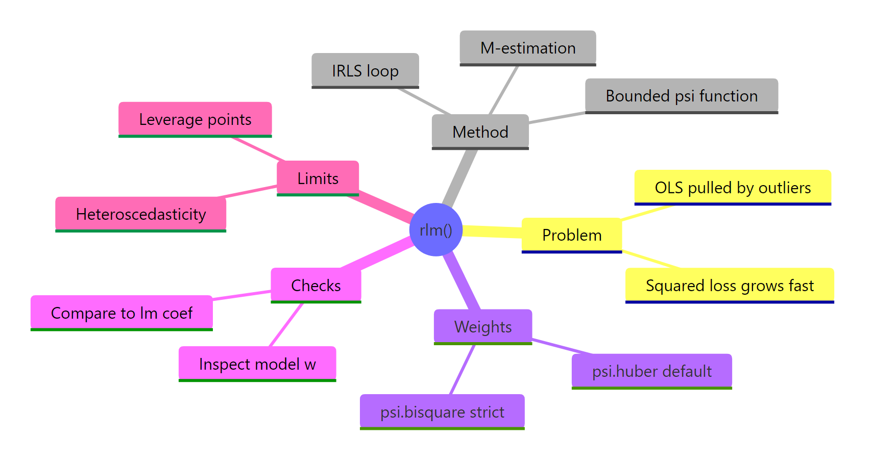
Figure 3: Robust regression at a glance: problem, method, weights, diagnostics, and limits.

The decision rule is simple. When you suspect your y values may contain a handful of extreme rows, fit rlm() alongside lm(). If they agree, your OLS fit is safe. If they diverge, sort rlm_fit$w ascending and inspect the outliers before reporting any coefficients to anyone.

References

Venables, W. N. & Ripley, B. D. Modern Applied Statistics with S, 4th edition (Springer, 2002). Chapter 8 covers rlm() and robust regression in depth. Book site
MASS package, rlm reference manual (CRAN). Documentation
Huber, P. J. (1964). Robust Estimation of a Location Parameter. Annals of Mathematical Statistics, 35(1), 73-101. JSTOR
Fox, J. & Weisberg, S. An R Companion to Applied Regression, 3rd edition (SAGE, 2019). Appendix on robust regression. Companion site
UCLA OARC Stats. Robust Regression R Data Analysis Examples. Tutorial
Maechler, M. et al. robustbase package (lmrob for MM-estimation). CRAN page
Wilcox, R. R. Introduction to Robust Estimation and Hypothesis Testing, 5th edition (Academic Press, 2021).

Continue Learning

Linear Regression Assumptions in R: the assumptions OLS leans on, and how to check them before reaching for robust alternatives.
Outlier Treatment With R: survey of detection methods (boxplots, Cook's distance, leverage) and remediation strategies before and after fitting.
Regression Diagnostics in R: the standard diagnostic plot toolkit (residuals, leverage, scale-location) that pairs naturally with rlm() weight inspection.

Robust Regression in R: Use rlm() When Outliers Are Ruining Your lm() Estimates

Why does one outlier wreck OLS, and what does rlm() do instead?

How does M-estimation downweight outliers?

When should you use Huber vs bisquare weights?

How do you find which points rlm() flagged as influential?

What are the limits of robust regression?

Practice Exercises

Exercise 1: Stackloss benchmark

Exercise 2: Contamination sweep

Complete Example

Summary

References

Continue Learning

Related Tutorials