Quantile Regression in R: quantreg Package, Model Beyond the Mean
Quantile regression, fit in R with the quantreg package's rq() function, models the conditional median (or any other quantile) of an outcome instead of its mean. It reveals how predictors act on low, typical, and high responses, captures heteroscedasticity, and resists outliers.
When should you reach for quantile regression instead of lm()?
Decisions about rent caps, hospital stay limits, or insurance premiums care about the tails, not just the average. Ordinary least squares collapses every bit of variability onto a single line through the mean, hiding the fact that one predictor may barely shift the median yet stretch the upper quartile sharply upward. Quantile regression, introduced by Koenker and Bassett (1978), traces that behaviour quantile by quantile.
The classic example ships inside quantreg itself: Engel's 1857 study of how food expenditure depends on household income. Fit the median regression with rq() and the mean regression with lm(), then compare.
The median slope (0.56) is steeper than the mean slope (0.49), and the median intercept is lower. That gap is not noise. Richer households spread their food spending further above the line than poorer households pull it below, so the mean gets tugged toward the high earners. The median tracks the typical household, which is what many policy decisions actually need.
Try it: Fit rq() at the median for Ozone ~ Solar.R on airquality (drop NAs first), then fit lm() on the same data. Compare the Solar.R slope at the mean vs median.
Click to reveal solution
Explanation: High-ozone days drag the OLS slope upward. The median slope is smaller because it describes the typical day, not the polluted outliers.
How does rq() fit a quantile instead of a mean?
OLS finds the line that minimises the sum of squared residuals. That loss treats positive and negative errors symmetrically, so the solution lands on the conditional mean. Quantile regression swaps squared loss for an asymmetric absolute loss called the check function. By tilting the penalty, it pushes the fit toward any quantile you name.
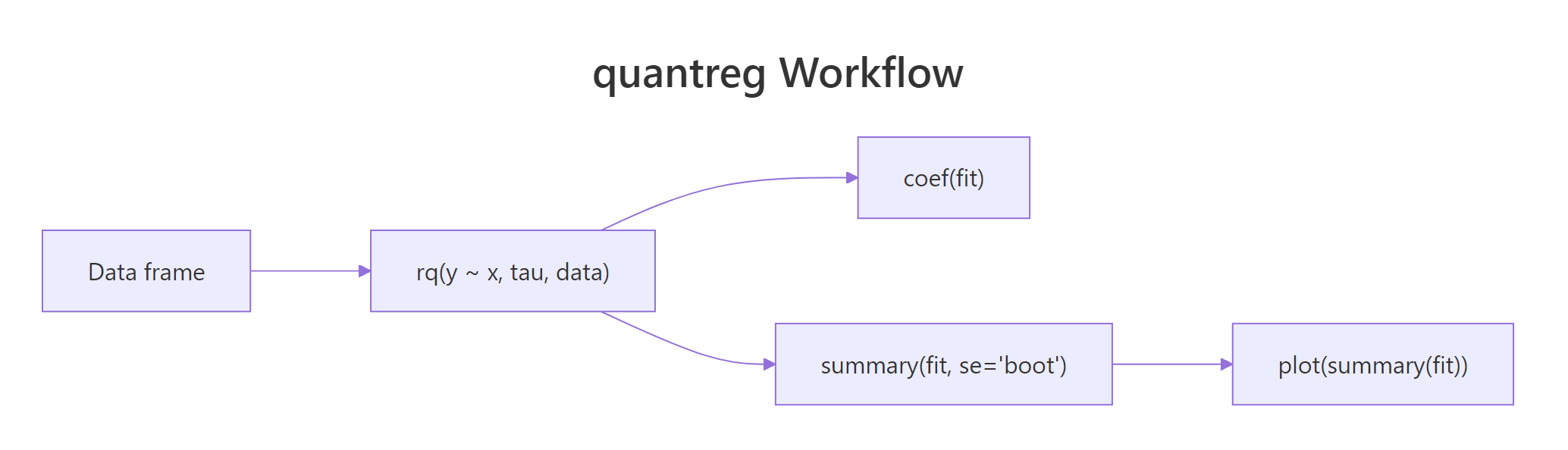
Figure 1: The quantreg workflow, fit with rq(), inspect coefficients, bootstrap standard errors, then plot the process.
The check function for quantile $\tau$ is:
$$\rho_\tau(u) = u \cdot (\tau - \mathbb{1}(u < 0))$$
Where:
- $u$ = the residual ($y - \hat{y}$)
- $\tau$ = the target quantile, between 0 and 1
- $\mathbb{1}(u < 0)$ = 1 when the residual is negative, 0 otherwise
At $\tau = 0.5$, both positive and negative residuals get weight 0.5, which recovers least absolute deviations (median regression). At $\tau = 0.9$, positive residuals get weight 0.9 and negative residuals get weight 0.1, so the fit pushes up until only 10% of observations sit above it. The optimiser solves a linear programme under the hood, which is why rq() handles any tau without Newton iterations.
Feeding a vector of taus to rq() fits all of them at once:
The income slope rises from 0.40 at the 10th percentile to 0.69 at the 90th, a 70% increase. That tells you high-spending households scale their food bill with income much more aggressively than frugal households do. OLS returns a single number (0.49) and forfeits this story.
Try it: Fit rq() at tau = 0.95 on the Engel data and interpret the intercept, how much does a household at the 95th percentile of food spending pay when income is at its lowest observed value?
Click to reveal solution
Explanation: The intercept 119 is the predicted food expenditure at income = 0 for the 95th percentile. It is larger than the median intercept (81), reflecting that the upper-tail line sits higher. The slope also grows, so rich households at the top of the spending distribution increase expenditure fastest.
How do you read the coefficients at different quantiles?
A coefficient at tau = 0.9 says: "if x increases by 1, the 90th percentile of y increases by this much." It does not say anything about the average household, only the one sitting at that specific quantile of the conditional distribution.
When slopes differ across taus, the effect of x is heterogeneous: it acts on low, middle, and high responders differently. When slopes are close to constant across taus, the effect is homogeneous and OLS is telling the whole story.
Scanning the income row, the slope climbs monotonically from 0.40 to 0.69. That monotonic rise is the signature of location-scale heterogeneity: both the mean and the spread of foodexp grow with income. If you cared about policy for the poorest 10%, 0.40 is your elasticity, not the OLS 0.49.
Try it: Fit rq() on mtcars for mpg ~ wt at tau = c(0.25, 0.5, 0.75). Does the weight penalty on fuel economy look uniform or heterogeneous across quantiles?
Click to reveal solution
Explanation: The wt slope hovers near -4.7 to -5.3 across quartiles, so weight hurts fuel economy fairly uniformly. No strong heterogeneity here, which means OLS would suffice for mean-focused questions.
How do you get reliable standard errors and confidence intervals?
summary(fit) returns confidence intervals by default, but the method matters because heteroscedasticity breaks simple formulas. The se argument of summary.rq() lets you choose:
se = value |
When to use |
|---|---|
"rank" (default) |
Small n; inverts a rank test; no nuisance parameters |
"iid" |
Residuals roughly iid and roughly symmetric |
"nid" |
Near-iid under heteroscedasticity; fast asymptotic |
"boot" |
Heteroscedastic or skewed data, most robust |
"ker" |
Kernel-based; similar intent to "nid" |
When in doubt, bootstrap. It makes no distributional assumptions and handles heteroscedasticity naturally.
The bootstrap standard error for income (0.033) gives a 95% confidence interval of roughly $[0.495, 0.625]$, so the median elasticity is estimated to about two decimal places. The rank-based default would sometimes return narrower intervals, but those can undercover under heteroscedasticity, so the bootstrap is the safer default on real data.
R = 200 is fine for exploration, but publish-ready numbers want 500 to 1000 resamples. Costly for large n, so downsample predictors first if needed.Try it: Compute bootstrap standard errors for fit_med using R = 300. Report the standard error of the income slope.
Click to reveal solution
Explanation: The income SE (~0.031) is close to the R=500 run (0.033), confirming 300 replicates already stabilise the estimate for this modest dataset.
How do you visualize effects across the entire distribution?
Reading coefficients at three taus is fine, but the richer picture is a quantile process plot, one panel per predictor showing the coefficient as a continuous function of tau. The dashed horizontal line marks the OLS estimate, and the shaded band is the confidence interval.
Fit rq() at a fine grid of taus, wrap the fit in summary() (bootstrap SE recommended), then pipe to plot().
Two panels appear, one for the intercept and one for the income slope. The income slope curve rises steadily from about 0.40 to 0.70 as tau moves from 0.05 to 0.95, well outside the OLS line for most of its range. That visible upward slope is the signature of conditional scale heterogeneity. A flat band hugging the OLS line would say "OLS is enough"; a tilted band, like this one, says "quantile regression is worth the extra work."
tau = seq(.05, .95, by = .05) or similar, not a random vector. The plot's x-axis is a density of quantile levels, not ordinal categories.Try it: Build a process plot for Engel with an added log-transformed income predictor. Which panel has the steepest tilt?
Click to reveal solution
Explanation: The log(income) panel captures the curvature and often has a more pronounced tilt across tau than the raw income panel, indicating the elasticity itself drifts across the distribution.
How does quantile regression expose heteroscedasticity?
Classical regression detects non-constant variance with a residual-vs-fitted plot: a visible funnel means the spread grows with x. Quantile regression offers a quantitative alternative. If the slope at tau=0.9 exceeds the slope at tau=0.1, the upper tail grows faster than the lower tail, a direct fingerprint of heteroscedasticity.
The 10th-percentile slope is 1.02 and the 90th-percentile slope is 1.98, almost double. The true generating process made residual SD proportional to $0.5 + 0.4x$, so the tails pull apart as x grows. Quantile regression reads this off directly: coef(fit)[2, "tau= 0.9"] - coef(fit)[2, "tau= 0.1"] estimates how much faster the upper tail climbs.
Try it: Generate a small dataset with constant variance (sd = 1, no dependence on x), fit rq() at tau=0.1 and 0.9, and confirm the slopes are close.
Click to reveal solution
Explanation: Both slopes cluster near the true 1.5, so the tails climb at the same rate. Variance is constant, quantile regression and OLS tell the same story about the conditional mean.
Practice Exercises
Exercise 1: Weight slope across mtcars quantiles
Fit rq() on mtcars for mpg ~ wt + cyl at tau = c(0.25, 0.5, 0.75). Extract the wt slope at each tau into a named numeric vector called my_wt_slopes.
Click to reveal solution
Explanation: Indexing coef(fit)["wt", ] pulls the wt row across all taus, the cleanest way to summarise a single predictor's behaviour across the distribution.
Exercise 2: Find the heterogeneous predictor on airquality
Fit rq() on na.omit(airquality) for Ozone ~ Solar.R + Wind + Temp at tau = c(0.1, 0.5, 0.9) with bootstrap SE (R = 300). Identify which predictor's slope changes the most between the 10th and 90th percentiles, assign the predictor name (string) to my_hetero.
Click to reveal solution
Explanation: Temperature's slope changes the most across quantiles, meaning hot days drive the upper ozone tail much more than they lift the lower tail, a heteroscedastic relationship the mean hides.
Exercise 3: Engel income elasticity at each decile
Fit rq() on Engel for foodexp ~ income at tau = seq(0.1, 0.9, by = 0.1). Return a data frame my_engel_decile with columns tau and income_slope.
Click to reveal solution
Explanation: The slope climbs monotonically from 0.40 to 0.69, quantifying how aggressively upper-decile households scale food spending with income. Policy analysts can quote the 10th-percentile elasticity when designing programmes for low-income families.
Complete Example
A full airquality workflow, from data cleaning to interpretation:
Reading the four panels (intercept plus three predictors): Temp climbs from 0.75 at tau=0.1 to 1.92 at tau=0.9, meaning each extra degree lifts the upper-tail ozone more than twice as much as the lower-tail ozone. Wind tilts steeply negative in the upper tail, so windy days clip the highest readings sharply. Solar.R shows modest heterogeneity, mostly a location shift. A single OLS model would have reported one average effect per predictor and hidden all three patterns.
Summary
Key takeaways from fitting quantile regression with quantreg:
| Step | Function | Purpose |
|---|---|---|
| Fit | rq(y ~ x, tau = ...) |
Estimate conditional quantile(s) |
| Inspect | coef(fit) |
Read slopes at each tau |
| Infer | summary(fit, se = "boot", R = 300+) |
Get bootstrap SEs robust to heteroscedasticity |
| Visualise | plot(summary(fit)) |
Process plot, coefficient vs tau |
| Diagnose | slope gap across taus | Heteroscedasticity fingerprint |
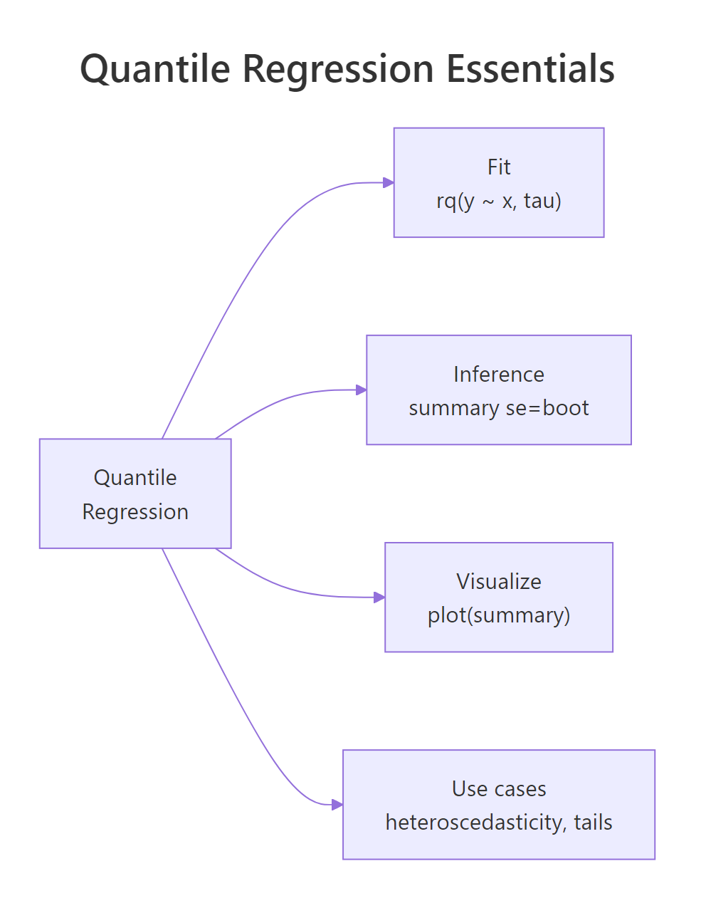
Figure 2: Quantile regression essentials, fit, inference, visualization, and core use cases.
Quantile regression earns its keep whenever the tails of the response matter, whenever variance changes with predictors, or whenever outliers corrupt OLS. For problems where the conditional mean is all you need and residual variance is constant, lm() remains simpler and sufficient. The quantreg package also extends beyond rq(): rqss() adds nonparametric smoothing, crq() handles censored responses, and nlrq() fits nonlinear quantile models.
References
- Koenker, R. & Bassett, G. (1978). Regression Quantiles. Econometrica, 46(1), 33-50. Link
- Koenker, R. & Hallock, K. (2001). Quantile Regression. Journal of Economic Perspectives, 15(4), 143-156. Link
- Koenker, R. (2005). Quantile Regression. Cambridge University Press.
- Koenker, R. quantreg package CRAN vignette. Link
- Cade, B. S. & Noon, B. R. (2003). A gentle introduction to quantile regression for ecologists. Frontiers in Ecology and the Environment, 1(8), 412-420. Link001%5B0412:AGITQR%5D2.0.CO%3B2)
- CRAN, Package 'quantreg' reference manual. Link
Continue Learning
- Polynomial and Spline Regression in R, the parent tutorial on modelling curvature without leaving the conditional mean.
- Linear Regression in R, the OLS baseline quantile regression generalises.
- Beta Regression in R, for bounded responses where neither OLS nor quantile regression is appropriate.