Regression Through the Origin in R: When to Force a Zero Intercept

Regression through the origin forces your linear model to pass through (0, 0) by dropping the intercept term. In R, you do it by writing lm(y ~ -1 + x) or lm(y ~ 0 + x). It is a tempting shortcut when theory says y must be zero at x = 0, but it changes how you should read almost every number summary() prints.

What does regression through the origin look like in R?

A standard lm() call fits two numbers, an intercept and a slope. A regression through the origin fits only the slope and assumes the line must pass through zero. Here is the one-character change that flips mtcars from "predict mpg from weight, with a non-zero baseline" to "predict mpg from weight, with no baseline at all":

RForce the intercept to zero on mtcars

# Drop the intercept with -1 in the formula m_ni <- lm(mpg ~ -1 + wt, data = mtcars) coef(m_ni) #> wt #> 5.291308

Look at that slope carefully. It is positive, 5.29 miles per gallon for every extra 1,000 lbs of car. Every car enthusiast knows heavier cars get worse mileage, not better. The standard model on the same data gives a slope of -5.34, with the expected sign. By forcing the line through (0, 0) we lost the freedom to set a sensible baseline, and the slope twisted to compensate. That is the warning shot: a no-intercept model can hand you a correct-looking number that is pointing the wrong way.

Try it: Fit a no-intercept model on iris for Sepal.Length ~ Petal.Length and print the slope.

RYour turn: no-intercept lm on iris

# Fit a no-intercept model with iris ex_model <- # your code here coef(ex_model) #> Expected: a single named number near 1.08

Click to reveal solution

Riris no-intercept solution

ex_model <- lm(Sepal.Length ~ -1 + Petal.Length, data = iris) coef(ex_model) #> Petal.Length #> 1.083558

Explanation: The -1 drops the intercept. The slope now absorbs whatever vertical offset the full model would have used, so it rarely matches the full-model slope.

How do you drop the intercept in R?

R gives you two equivalent syntaxes. -1 says "remove the intercept term." 0 + says "start the formula with zero, then add predictors." Both produce the same model.

R-1 and 0 + produce the same model

# Two ways to drop the intercept m_minus1 <- lm(mpg ~ -1 + wt, data = mtcars) m_zero <- lm(mpg ~ 0 + wt, data = mtcars) coef(m_minus1) #> wt #> 5.291308 coef(m_zero) #> wt #> 5.291308

Both coefficients match to six digits because they are fitting the same ordinary-least-squares problem. Pick whichever reads best in your formula.

Tip

Prefer 0 + in long formulas. When you have many predictors, lm(y ~ 0 + x1 + x2 + x3 + x4) makes the "no intercept" choice obvious from the left. -1 at the start or buried mid-formula is easier to miss during code review.

Multiple predictors work the same way. You are still fitting a single hyperplane that passes through the origin, with one slope per predictor:

RMulti-predictor no-intercept model

# Two predictors, no intercept m_ni_multi <- lm(mpg ~ 0 + wt + hp, data = mtcars) coef(m_ni_multi) #> wt hp #> 6.80690787 -0.03295617

With the intercept dropped, both slopes must explain all of mpg starting from zero. The wt coefficient bloats from 5.29 (single-predictor, no-intercept) to 6.81, and hp gets a small negative slope to pull predictions back down. The individual numbers stop lining up with the one-variable-at-a-time intuition you may carry from the full model.

Try it: Using the 0 + syntax, fit mpg ~ cyl + disp on mtcars without an intercept.

RYour turn: two-predictor no-intercept

# Fit mpg ~ cyl + disp with 0 + syntax ex_model2 <- # your code here coef(ex_model2) #> Expected: two coefficients, one for cyl, one for disp

Click to reveal solution

RTwo-predictor no-intercept solution

ex_model2 <- lm(mpg ~ 0 + cyl + disp, data = mtcars) coef(ex_model2) #> cyl disp #> 3.82015301 0.01225919

Explanation: Both predictors now share the job of explaining mpg without any constant term. The cyl coefficient is large because it absorbs what the full model's intercept would have captured.

When does forcing a zero intercept actually make sense?

The honest answer: less often than you think. There are a few clean cases where it genuinely fits:

Calibration curves in analytical chemistry, where absorbance is physically zero at concentration zero (blank reading subtracted).
Ratio-scale physical relationships: distance = speed × time when time is measured from a stop, voltage = current × resistance, mass = density × volume.
Comparison of two measurement devices when both report the same physical quantity on a ratio scale and you want the slope to be the conversion factor.
Dose-response in settings where a true blank exists, and the response is defined as zero at zero dose.

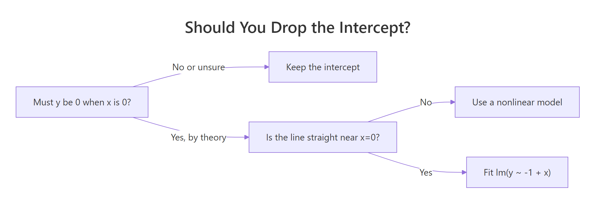
Decide in three questions whether dropping the intercept is safe.

Figure 1: Decide in three questions whether dropping the intercept is safe.

Key Insight

The real question is whether the line is straight all the way to x = 0. Knowing the true intercept is zero is not enough. Your linear form must also be correct near the origin. If the relationship curves near zero (saturation, thresholds), a no-intercept line will fit one part of the range well and lie elsewhere.

Here is a synthetic calibration problem where a no-intercept model is the right call. We simulate 20 standards with true slope 2.5 and genuine zero intercept, then fit both models:

RCalibration simulation with true zero intercept

# Simulate a calibration curve: y = 2.5*x + noise, true intercept is 0 library(ggplot2) set.seed(71) x_conc <- seq(0.1, 5, length.out = 20) y_abs <- 2.5 * x_conc + rnorm(20, sd = 0.2) cal_df <- data.frame(concentration = x_conc, absorbance = y_abs) m_cal <- lm(absorbance ~ 0 + concentration, data = cal_df) m_cal_full <- lm(absorbance ~ concentration, data = cal_df) coef(m_cal) #> concentration #> 2.506408 coef(m_cal_full) #> (Intercept) concentration #> 0.04012103 2.4907833

The no-intercept slope lands at 2.506, essentially bang on the true value of 2.5. The full model's intercept is 0.04, statistically indistinguishable from zero given this noise, and its slope (2.491) is a hair farther from the truth. In this case dropping the intercept spends the extra degree of freedom usefully. Contrast this with mtcars where the no-intercept slope flipped sign: the difference is that here the line actually is straight down to zero.

Try it: Which of these scenarios should use regression through the origin? A, B, or both?

A. Predicting monthly grocery spend from household size. B. Predicting absorbance from concentration in a lab assay, with a blank-subtracted sensor.

RYour turn: pick the right scenario

# Write "A", "B", or "both" ex_answer <- "___" ex_answer #> Expected: "B"

Click to reveal solution

RScenario solution

ex_answer <- "B" ex_answer #> [1] "B"

Explanation: A household of size zero is a meaningless extrapolation, and grocery spend is not known to be zero there. Scenario B has a blank-subtracted sensor where zero concentration is defined to produce zero absorbance. Only B satisfies the "line is straight down to zero" rule.

Why is R-squared misleading when you drop the intercept?

This is the trap. The R² that summary() prints for a no-intercept model is computed with a different total sum of squares than the one for a full model, and the two numbers are not comparable.

For a full model, R² is:

$$R^2 = 1 - \frac{\sum (y_i - \hat{y}_i)^2}{\sum (y_i - \bar{y})^2}$$

For a no-intercept model, R computes:

$$R^2_{\text{uncentered}} = 1 - \frac{\sum (y_i - \hat{y}_i)^2}{\sum y_i^2}$$

The denominator changed from "variation around the mean" to "squared distance from zero." The second denominator is much larger whenever your y values are far from zero, so the reported R² looks flattering even when the fit is awful.

Watch this happen on the mtcars model we fit at the top:

RReported R-squared vs true centered R-squared

# lm reports this R-squared summary(m_ni)$r.squared #> [1] 0.7196604 # Compute the centered R-squared by hand y_mt <- mtcars$mpg yhat_mt <- predict(m_ni) ss_res <- sum((y_mt - yhat_mt)^2) ss_tot_cen <- sum((y_mt - mean(y_mt))^2) r2_centered <- 1 - ss_res / ss_tot_cen r2_centered #> [1] -2.495960

The reported R² of 0.72 is a siren song. Compute the same quantity with the centered baseline that every regression textbook uses, and you get −2.50. Negative. The no-intercept model is worse than just predicting every car's mpg as the dataset mean. Meanwhile, summary() keeps happily printing 0.72 as if nothing were wrong.

Warning

Never compare R-squared across with- and without-intercept models. R reports them on different scales. If you need a fair comparison, refit both models and compute the centered R² yourself, or compare them on residual sum of squares or RMSE, which are on the same units either way.

Try it: Compute the centered R² for lm(Petal.Length ~ -1 + Sepal.Length, data = iris) and compare it with what summary() reports.

RYour turn: centered R-squared on iris

ex_m <- lm(Petal.Length ~ -1 + Sepal.Length, data = iris) # Reported ex_r2_reported <- summary(ex_m)$r.squared # Centered (compute yourself) ex_r2_centered <- # your code here c(reported = ex_r2_reported, centered = ex_r2_centered) #> Expected: reported ~0.94, centered ~0.43

Click to reveal solution

Riris centered R-squared solution

ex_m <- lm(Petal.Length ~ -1 + Sepal.Length, data = iris) ex_r2_reported <- summary(ex_m)$r.squared ex_y <- iris$Petal.Length ex_r2_centered <- 1 - sum((ex_y - predict(ex_m))^2) / sum((ex_y - mean(ex_y))^2) c(reported = ex_r2_reported, centered = ex_r2_centered) #> reported centered #> 0.9381831 0.4301063

Explanation: Reported 0.94 sounds excellent. Centered 0.43 tells the honest story: on the textbook scale this model only explains 43% of the variation around the mean.

How do predictions compare with and without intercept?

The cleanest diagnostic is a plot. Fit both models, draw both lines, see where they disagree. On mtcars the story is immediate:

RPlot full-model and no-intercept fits together

# Fit both models and overlay their fits on a scatter m_full <- lm(mpg ~ wt, data = mtcars) ggplot(mtcars, aes(x = wt, y = mpg)) + geom_point(size = 2) + geom_abline(intercept = coef(m_full)[1], slope = coef(m_full)[2], colour = "steelblue", linewidth = 1) + geom_abline(intercept = 0, slope = coef(m_ni)[1], colour = "firebrick", linewidth = 1, linetype = "dashed") + labs(title = "mtcars: full model (blue) vs no-intercept (red dashed)", x = "Weight (1000 lbs)", y = "Miles per gallon") + theme_minimal()

The blue line tilts downward through the cloud of points like you would expect. The red dashed line starts at the origin and slopes upward, missing the data entirely at both ends. That picture is worth more than any R² table.

Note

Always plot both fits before choosing. Residual plots or a simple scatter with two overlays will reveal a misspecified no-intercept model faster than any summary statistic, including BIC or AIC.

Numerically, the gap between the two models grows with the distance from zero. Predicting mpg for a medium-weight car makes the point:

RPredict for a new 3,000 lb car under both models

# Same car, two predictions new_car <- data.frame(wt = 3.0) pred_full <- predict(m_full, new_car) pred_ni <- predict(m_ni, new_car) c(full = pred_full, no_intercept = pred_ni) #> full.1 no_intercept.1 #> 21.25171 15.87392

A 5.4 mpg gap between two models fit to the same 32 data points. The full model is close to the actual average mpg at wt = 3 (around 20). The no-intercept model is five miles per gallon low because its forced-through-origin line starts too low and climbs the wrong way.

Try it: Predict mpg at wt = 2.0 under both models and compute the difference.

RYour turn: predict at wt = 2.0

ex_new <- data.frame(wt = 2.0) ex_full <- predict(m_full, ex_new) ex_ni <- # your code here c(full = ex_full, no_intercept = ex_ni, diff = ex_full - ex_ni) #> Expected: the no-intercept prediction is much lower than the full-model one

Click to reveal solution

RPredict at wt = 2.0 solution

ex_new <- data.frame(wt = 2.0) ex_full <- predict(m_full, ex_new) ex_ni <- predict(m_ni, ex_new) c(full = ex_full, no_intercept = ex_ni, diff = ex_full - ex_ni) #> full.1 no_intercept.1 diff.1 #> 26.596141 10.582615 16.013526

Explanation: At wt = 2, the full model predicts 26.6 mpg. The no-intercept model predicts 10.6, less than half, because its forced-zero line is climbing from the origin rather than fitting the actual data range.

Practice Exercises

Exercise 1: Fit and compare on the `cars` dataset

A physicist argues that a car at zero speed should take zero feet to stop, so a no-intercept model for dist ~ speed must be correct. Fit both models on the built-in cars dataset. Report the RMSE of each on the training data. Which model has lower RMSE, and do you agree with the physicist's reasoning after seeing the numbers?

RExercise 1: full vs no-intercept on cars

# Fit both models and compute RMSE for each # Hint: RMSE = sqrt(mean(residuals(model)^2)) my_full <- # ... my_ni <- # ... rmse_full <- # ... rmse_ni <- # ... c(full = rmse_full, no_intercept = rmse_ni) #> Expected: RMSE values around 15 for each model

Click to reveal solution

RExercise 1 solution

my_full <- lm(dist ~ speed, data = cars) my_ni <- lm(dist ~ 0 + speed, data = cars) rmse_full <- sqrt(mean(residuals(my_full)^2)) rmse_ni <- sqrt(mean(residuals(my_ni)^2)) c(full = rmse_full, no_intercept = rmse_ni) #> full no_intercept #> 15.06886 15.93897

Explanation: The no-intercept model has marginally worse RMSE, which is a hint that the physicist's clean "zero at zero" story is not the whole picture. Stopping distance includes reaction-time distance that is roughly constant, so the true intercept is not exactly zero in the observed regime. The full model's negative intercept (around -17) is not physically meaningful but does compensate for a linear form that is mildly wrong near zero.

Exercise 2: Compare slope confidence intervals on simulated data

Simulate 30 points from y = 3*x + noise with x = seq(1, 10, length.out = 30) and noise of standard deviation 2. Fit both a full model and a no-intercept model. Extract the 95% confidence interval for the slope from each. Do the intervals overlap?

RExercise 2: slope CIs on simulated data

set.seed(2026) my_x <- seq(1, 10, length.out = 30) my_y <- 3 * my_x + rnorm(30, sd = 2) my_df <- data.frame(x = my_x, y = my_y) # Fit both models and get slope CIs with confint() # Hint: confint(model)["x", ] returns the slope CI row my_ci_full <- # ... my_ci_ni <- # ... list(full = my_ci_full, no_intercept = my_ci_ni) #> Expected: both intervals bracket 3, no-intercept interval tends to be narrower

Click to reveal solution

RExercise 2 solution

set.seed(2026) my_x <- seq(1, 10, length.out = 30) my_y <- 3 * my_x + rnorm(30, sd = 2) my_df <- data.frame(x = my_x, y = my_y) my_fit_full <- lm(y ~ x, data = my_df) my_fit_ni <- lm(y ~ 0 + x, data = my_df) my_ci_full <- confint(my_fit_full)["x", ] my_ci_ni <- confint(my_fit_ni)["x", ] list(full = my_ci_full, no_intercept = my_ci_ni) #> $full #> 2.5 % 97.5 % #> 2.848614 3.257147 #> #> $no_intercept #> 2.5 % 97.5 % #> 2.926601 3.141498

Explanation: Both intervals bracket the true slope of 3. The no-intercept interval is tighter because it spends zero degrees of freedom estimating the intercept. The trade-off only pays off because the data genuinely pass through the origin. On real data where you are not sure, the narrower interval is a false comfort.

Exercise 3: Explain the R-squared gap on mtcars

Using m_ni from earlier in the tutorial, show in code that summary(m_ni)$r.squared equals 1 - sum(residuals(m_ni)^2) / sum(mtcars$mpg^2), confirming the uncentered denominator. Then write a one-sentence explanation of why the centered R² is so much lower.

RExercise 3: derive lm's reported R-squared

# Hint: sum(y^2) is the uncentered total sum of squares ss_res_ni <- # ... ss_tot_uncentered <- # ... reported <- summary(m_ni)$r.squared by_formula <- # ... c(reported = reported, by_formula = by_formula) #> Expected: both numbers equal ~0.7197

Click to reveal solution

RExercise 3 solution

ss_res_ni <- sum(residuals(m_ni)^2) ss_tot_uncentered <- sum(mtcars$mpg^2) reported <- summary(m_ni)$r.squared by_formula <- 1 - ss_res_ni / ss_tot_uncentered c(reported = reported, by_formula = by_formula) #> reported by_formula #> 0.7196604 0.7196604

Explanation: The reported R² uses sum(y^2) in the denominator instead of sum((y - mean(y))^2). On mtcars, mpg averages around 20, so squared distances from zero are much larger than squared distances from the mean. That inflated denominator makes the fraction of "variation explained" look artificially high even though the model misses the centered target badly.

Complete Example: A spectrophotometer calibration curve

Here is the flow you would actually use in a lab. We simulate ten calibration standards where absorbance is known to be zero at zero concentration (the instrument was blank-corrected), fit a no-intercept model because the linear form is trustworthy down to the origin, and use it to estimate the concentration of an unknown sample.

RSimulate calibration data

# Ten standards with known concentrations and measured absorbance set.seed(310) std_conc <- c(0.1, 0.2, 0.5, 1.0, 1.5, 2.0, 2.5, 3.0, 4.0, 5.0) std_abs <- 1.82 * std_conc + rnorm(10, sd = 0.04) lab_df <- data.frame(concentration = std_conc, absorbance = std_abs) head(lab_df, 4) #> concentration absorbance #> 1 0.1 0.1521147 #> 2 0.2 0.3815216 #> 3 0.5 0.9113135 #> 4 1.0 1.8128119

Tip

Pair every calibration fit with a residual plot. A residual-vs-concentration plot that shows a trumpet shape or curvature tells you the linear form is wrong, even when the slope and R² look fine.

Now fit the calibration line through the origin and predict an unknown sample whose absorbance came out at 1.63:

RFit calibration and predict an unknown

# Fit through origin, predict concentration for an unknown absorbance m_lab <- lm(absorbance ~ 0 + concentration, data = lab_df) summary(m_lab)$coefficients #> Estimate Std. Error t value Pr(>|t|) #> concentration 1.821354 0.006931923 262.7596 1.196657e-18 # An unknown sample reads 1.63 absorbance units # Invert the calibration line: concentration = absorbance / slope unknown_abs <- 1.63 unknown_conc <- unknown_abs / coef(m_lab)[["concentration"]] unknown_conc #> [1] 0.8948300

The slope of 1.821 is the molar absorptivity estimate, and its standard error is tiny because we have ten well-spaced standards. Inverting the fit gives an estimated concentration of 0.895 for the unknown sample. Because the model passes through the origin by construction, we do not have to worry about whether a small intercept estimate near zero is signal or noise. This is regression through the origin working the way it is meant to.

RPlot the calibration line

# Visualize the fit ggplot(lab_df, aes(x = concentration, y = absorbance)) + geom_point(size = 3, colour = "steelblue") + geom_abline(intercept = 0, slope = coef(m_lab)[1], colour = "firebrick", linewidth = 1) + labs(title = "Spectrophotometer calibration (zero intercept)", x = "Concentration (mM)", y = "Absorbance") + theme_minimal()

The line starts at (0, 0) and cuts through every point. That is what a valid regression through the origin looks like. Compare the shape of this plot with the mtcars red-dashed line earlier, which missed the data cloud entirely.

Summary

The short version: forcing your regression through the origin is a modelling decision, not a default. The table below is the shortlist of when to use it and when to leave the intercept in.

Situation	Force zero intercept?
Calibration curve with blank-subtracted sensor	Yes
Physical laws: distance = rate × time, V = IR	Yes
Comparison of two measurements of the same ratio-scale quantity	Yes
Theory says intercept is zero but data never near x = 0	No (linear form unverified near zero)
You want a tighter slope CI	No (borrowed certainty, not real)
You want a higher R²	No (different denominator, not a fair comparison)
You have not plotted the data	No (plot first, decide after)

Key Insight

An estimated intercept far from zero is a diagnostic, not a problem to paper over. It is telling you either that the true intercept is not actually zero in your data range, or that your linear form is bending near the origin. Forcing the line through (0, 0) silences that signal without fixing it.

Three takeaways:

The R syntax is simple: lm(y ~ -1 + x) or lm(y ~ 0 + x). The decision is the hard part.
summary()'s R² uses a different denominator for no-intercept models. It is not comparable across the two model types. Compute a centered R² by hand if you need to compare.
Plot both fits. A two-line overlay tells you in five seconds what a table of statistics can hide.

References

Eisenhauer, J. G. (2003). Regression through the Origin. Teaching Statistics, 25(3), 76–80. Link
Casella, G. (1983). Leverage and regression through the origin. The American Statistician, 37(2), 147–152. Link
R Core Team. *lm() documentation, including formula syntax*. Link
Fox, J. (2017). Don't force your regression through zero just because you know the true intercept has to be zero. Dynamic Ecology. Link
SAS Communities Library. The Why, How, and Cautions of Regression Without an Intercept. Link

Continue Learning

Linear Regression Assumptions in R, the assumption set lm() relies on and which assumptions shift when you drop the intercept.
Regression Diagnostics in R, the residual plots that expose a misspecified no-intercept model faster than any fit statistic.
Multicollinearity in R, another silent regression pitfall that also inflates fit statistics without flagging itself.

Regression Through the Origin in R: When to Force a Zero Intercept

What does regression through the origin look like in R?

How do you drop the intercept in R?

When does forcing a zero intercept actually make sense?

Why is R-squared misleading when you drop the intercept?

How do predictions compare with and without intercept?

Practice Exercises

Exercise 1: Fit and compare on the cars dataset

Exercise 2: Compare slope confidence intervals on simulated data

Exercise 3: Explain the R-squared gap on mtcars

Complete Example: A spectrophotometer calibration curve

Summary

References

Continue Learning

Related Tutorials

Exercise 1: Fit and compare on the `cars` dataset