Multiple Regression in R: How to Build, Interpret, and Refine a Real Model

Multiple regression in R extends lm() to include more than one predictor, so each coefficient measures the independent effect of its variable while holding the others constant. This lets you separate the real signal from confounders and build a model that actually generalizes.

This tutorial uses base R plus a touch of dplyr and ggplot2. Every code block runs in your browser, so you can edit a formula and rerun without leaving this page.

When does a single predictor lie to you?

Predicting mpg from wt alone on the mtcars dataset gives you one slope. Add hp and qsec to the model and every coefficient shifts, because each predictor now has to earn its keep after the others explain what they can. That is the whole point of multiple regression, and you can see the shift in a single lm() call.

Run the block below to fit a 3-predictor model on mtcars and read its summary table.

The model explains roughly 82% of the variance in fuel economy (adjusted R²). Each kilo of weight (wt is in thousand-pound units) drops mpg by about 4.4 miles per gallon, holding hp and qsec constant. The other two coefficients are in the right direction but their p-values say we can't distinguish them from noise once wt is in the model. That is already a useful real-world conclusion: when you control for weight, raw horsepower stops looking like the main mileage killer.

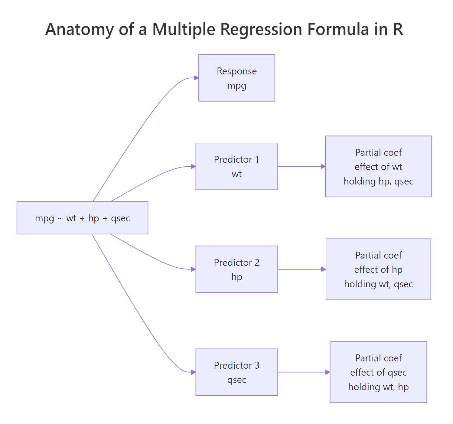
Figure 1: Each term on the right-hand side of the formula contributes one partial coefficient.

How do you read the partial coefficients?

"Holding the other predictors constant" sounds like a textbook caveat, but it is literally the mechanism that changes the numbers. Fit the same predictor on its own and again with another predictor next to it, and the coefficient will shift whenever the two predictors share information.

The slope on wt collapsed from -5.34 to -3.88 once hp joined the model. That happened because heavier cars tend to have more horsepower, so the simple model was crediting wt for an effect that really came from both. Multiple regression splits the credit. This is the partial-coefficient idea in action and the reason you cannot interpret coefficients in isolation.

Once you trust the model, you can use it to predict mpg for a new car. predict() gives you the point estimate; passing interval = "confidence" adds a confidence band for the mean response at that combination of inputs.

The model expects a car with these specs to deliver about 21.3 mpg, and we are 95% confident the average mpg for cars with this profile lies between roughly 19.8 and 22.8.

How do you tell which predictors actually matter?

The summary table from lm() is built for this question. Read it column by column: Estimate is the coefficient, Std. Error is its standard error, t value is Estimate ÷ Std. Error, and Pr(>|t|) is the p-value testing whether the true coefficient is zero. Stars are a quick visual cue for that p-value.

For machine-readable output, pull just the coefficient table and add confint() to bracket each estimate with a 95% confidence interval.

Two things to read at a glance: only wt's confidence interval excludes zero, which is why only wt is statistically significant. The intervals for hp and qsec straddle zero, which is the same story the p-value told you. The bottom line of the full summary(), the F-statistic, asks a different question: is the whole model better than an intercept-only model? Here the F p-value is essentially zero, so the model as a whole is useful even though two of its three predictors aren't pulling weight individually.

Fit a wider model and you can find a predictor that fails the test outright.

drat and gear both have p-values around 0.5–0.6 and tiny t-values, which makes them the obvious candidates to drop.

How do you add categorical predictors (factors)?

Categorical variables enter the formula as factors. R automatically expands a factor with k levels into k-1 dummy variables. Each dummy's coefficient is the average difference from the reference level, holding the other predictors constant.

Start with am, which is 0 (automatic) or 1 (manual) in mtcars. Convert it to a factor inline so R treats it categorically rather than numerically.

The intercept is the predicted mpg for an automatic car with wt = 0, which is a useful anchor even though no real car weighs zero. factor(am)1 is the average bump for manual cars over automatics at the same weight, which here is essentially zero. The data is telling you that once you control for weight, transmission stops mattering, even though raw mpg differs noticeably between manuals and automatics.

A factor with three or more levels produces multiple dummies, one per non-reference level.

The reference level is 4-cylinder (the lowest level by default). factor(cyl)6 says a 6-cylinder car gets about 4.3 mpg less than a 4-cylinder car at the same weight. The 8-cylinder penalty is even larger at about 6.1 mpg.

Now the dummies measure how much better a 4- or 6-cylinder car is than an 8-cylinder car at the same weight. The 6.07 mpg gain for 4-cylinder over 8-cylinder is exactly the mirror image of the -6.07 you saw before; the model is the same fit, just relabeled.

How do you refine the model by dropping weak predictors?

A clean refinement workflow beats blind stepwise selection. The recipe: fit the wide model, drop the predictor with the highest p-value, refit, and check that adjusted R² did not drop in any meaningful way. Repeat until every survivor is justified.

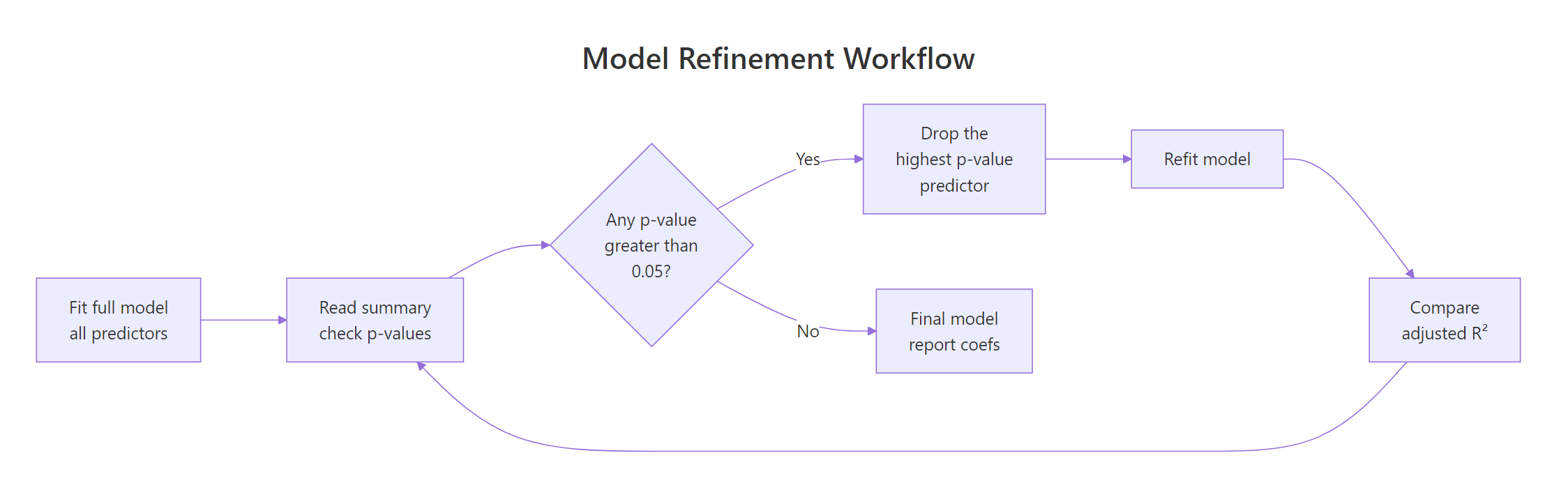
Figure 2: Drop the predictor with the highest p-value, refit, and watch adjusted R² before committing.

Recall model_full from earlier had gear with the largest p-value. Drop it and compare.

Adjusted R² actually went up slightly (0.808 to 0.814). That is the signal that gear was hurting more than it helped; once it leaves, the remaining predictors absorb its variance more efficiently. Now you can compare the two models formally with anova().

The F-test compares the residual sum of squares between the two nested models. A p-value of 0.64 means the wider model does not fit significantly better, so dropping gear was the right call.

How do you rank predictor importance with standardized coefficients?

Raw coefficients live in different units. wt is in thousands of pounds, hp is in horsepower, qsec is in seconds. You cannot compare -4.4 (per 1000 lb) to -0.018 (per horsepower) and conclude one matters more. To rank importance, put every predictor (and the response) on a common scale by standardizing them: subtract the mean and divide by the standard deviation. Now every coefficient is in standard-deviation units.

The intercept is exactly zero (a side effect of standardizing) and the partial coefficients are now directly comparable. A 1-SD increase in wt drops mpg by about 0.66 SD, holding hp and qsec constant. By absolute value, wt is roughly 5 times more impactful than hp and 5 times more than qsec. That is the kind of comparison the unscaled model cannot give you.

How do you add interaction effects?

So far every coefficient has measured an effect that is the same at every level of every other predictor. Sometimes that assumption is wrong. The slope of mpg on wt may genuinely differ between automatic and manual cars; that is what an interaction captures.

Use * in the formula to fit both main effects and the interaction in one shot. wt * factor(am) is shorthand for wt + factor(am) + wt:factor(am).

Read the rows like this. For automatic cars (am = 0), the slope of mpg on wt is the bare wt coefficient: -3.79. For manual cars (am = 1), the slope is -3.79 + (-5.30) = -9.09. In other words, manuals lose mileage much faster as they get heavier than automatics do. Both effects are statistically significant, with p-values well under 0.01.

A picture makes this concrete. Color points by transmission and let ggplot2 fit a separate line per group.

The two regression lines visibly cross. Light cars do better with a manual transmission, heavy cars do better with an automatic. That crossover is the practical meaning of a significant interaction term, and it is the sort of insight a "no-interaction" multiple regression would miss entirely.

Practice Exercises

These capstone exercises mix multiple ideas from the tutorial. They use the prefix my_ to keep them isolated from the tutorial state above.

Exercise 1: Refine a 4-predictor model on mtcars

Fit a multiple regression of mpg on wt, hp, disp, and drat using mtcars. Drop the least significant predictor one at a time until every survivor has p < 0.10. Save the final model to my_final_model.

Exercise 2: Test whether species adds predictive value on iris

Using the iris dataset, fit Sepal.Length ~ Sepal.Width + Petal.Length + Petal.Width (call it my_no_species) and Sepal.Length ~ Sepal.Width + Petal.Length + Petal.Width + Species (call it my_with_species). Compare them with anova() and decide whether species contributes beyond the other predictors.

Exercise 3: Read the per-cylinder slope from an interaction

Fit mpg ~ wt * factor(cyl) on mtcars. Save the model to my_cyl_int. Report the wt slope separately for 4-, 6-, and 8-cylinder cars by combining the main effect with the relevant interaction term.

Putting It All Together

This walkthrough builds a multiple regression on mtcars end to end: fit a wide model, prune it down, standardize to rank importance, and add an interaction where the data calls for one. Each step uses only ideas covered above.

Three weak candidates jump out: drat, gear, and carb all have p-values above 0.5. Drop the worst, refit, repeat.

After three drops we are back to the model from section 1, with adjusted R² up to 0.817. wt is the only predictor with p < 0.05, but hp and qsec are theoretically defensible (engine power and acceleration matter for fuel economy), so keep them. Now standardize to compare their importance.

wt is roughly 5 times more impactful than the other two on a standardized basis. Finally, ask whether the relationship between wt and mpg actually depends on transmission type by adding an interaction.

The interaction term wt:factor(am)1 is highly significant, so transmission really does change the slope of mpg on wt even after controlling for hp and qsec. The full story now reads: weight is the dominant driver of fuel economy, horsepower and quarter-mile time contribute smaller but real effects, and that weight effect is much steeper for manuals than automatics. That is a more complete and more useful answer than the original "wt is significant" you would have gotten from a simple regression.

Summary

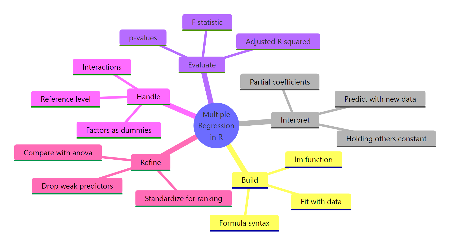
Figure 3: The five moves that turn an lm() call into a trustworthy multiple regression.

The five moves you now know:

1. Build with lm(). Use formula syntax y ~ x1 + x2 + x3 and pass the data frame.
2. Read coefficients as partial effects. Each coefficient is the effect of its predictor holding all the others fixed; the same variable's coefficient will shift as you add or drop other predictors.
3. Decode summary(). Look at coefficient size, p-value, adjusted R², and the F-statistic at the bottom for overall model significance.
4. Handle factors and interactions. Convert categorical predictors with factor(); use * for interactions when one predictor's effect plausibly depends on another.
5. Refine deliberately. Drop the highest-p-value predictor first, refit, watch adjusted R², and use anova() to formally compare nested models. Standardize to rank importance.

References

1. James, G., Witten, D., Hastie, T., & Tibshirani, R., An Introduction to Statistical Learning, 2nd Edition. Chapter 3: Linear Regression. Link
2. Wickham, H., & Grolemund, G., R for Data Science, 2nd Edition. Chapter on Model building. Link
3. R Core Team, lm() reference manual. Link
4. Dalgaard, P., Introductory Statistics with R, 2nd Edition. Chapter 11: Multiple regression. Springer.
5. Venables, W. N., & Ripley, B. D., Modern Applied Statistics with S (MASS), 4th Edition. Chapter 6: Linear statistical models. Springer.
6. Kutner, M. H., Nachtsheim, C. J., & Neter, J., Applied Linear Regression Models, 4th Edition. Chapters 6–7. McGraw-Hill.
7. UCLA Office of Advanced Research Computing, Regression with R. Link

Continue Learning

• Linear Regression in R, the single-predictor foundation that multiple regression generalizes.
• Linear Regression Assumptions in R, every diagnostic check your multiple regression model still needs.
• Logistic Regression in R, when the response variable is binary instead of continuous.