Effect Size in R: The Number p-Values Never Tell You (Cohen's d, η², and r)

Effect size measures the magnitude of a difference or association on a standardized, sample-size-free scale. Where p-values only tell you an effect probably exists, effect size tells you how large it is, so you know whether it matters in the real world.

Why does effect size matter more than p-values?

A p-value answers a narrow question: assuming no effect, how surprising is this data? But "statistically significant" is not the same as "practically important," especially in large samples where trivial differences reach p < 0.001. The fix is reporting effect size alongside every test. Here is the comparison that got buried when you only looked at the p-value.

Below, we compare fuel economy between automatic and manual transmissions in mtcars. The t-test returns a p-value. Then we compute Cohen's d, which converts the mean difference into units of pooled standard deviation, so we can judge how far apart the groups really are.

Rp-value versus Cohen's d on mtcars

# Split mpg by transmission: 0 = automatic, 1 = manual auto <- mtcars$mpg[mtcars$am == 0] manual <- mtcars$mpg[mtcars$am == 1] # 1. The usual p-value t.test(manual, auto)$p.value #> [1] 0.001373638 # 2. Cohen's d: mean difference in pooled-SD units n1 <- length(auto) n2 <- length(manual) s_pooled_mpg <- sqrt(((n1 - 1) * var(auto) + (n2 - 1) * var(manual)) / (n1 + n2 - 2)) d_mpg <- (mean(manual) - mean(auto)) / s_pooled_mpg round(d_mpg, 3) #> [1] 1.478

The p-value (0.0014) just tells you the difference is not pure noise. Cohen's d (1.48) tells you manuals average 1.48 pooled standard deviations higher than automatics in this dataset, which is a very large effect by any convention. Two numbers, two different questions answered.

Now watch what happens when the effect is tiny but the sample is huge. Big N shrinks standard errors, which shrinks p-values, even when the real difference is irrelevant.

RLarge N makes trivial differences significant

set.seed(42) # Two groups barely differ (true mean gap = 0.1), but n is 10000 each group_a <- rnorm(10000, mean = 10.0, sd = 2) group_b <- rnorm(10000, mean = 10.1, sd = 2) # p-value screams "significant" t.test(group_a, group_b)$p.value #> [1] 0.0003791061 # Cohen's d reveals the effect is basically nothing s_pooled_bigN <- sqrt(((10000 - 1) * var(group_a) + (10000 - 1) * var(group_b)) / (20000 - 2)) d_bigN <- (mean(group_b) - mean(group_a)) / s_pooled_bigN round(d_bigN, 3) #> [1] 0.052

The p-value says "reject the null." The effect size says "the gap is about 0.05 standard deviations, which no one would call meaningful." This is the classic N-inflated significance trap, and it is why every major journal now requires effect sizes alongside p-values.

Key Insight

Sample size changes p-values, not effect size. Doubling N roughly halves a p-value without changing d, η², or r. That is why effect size is the number that tells you whether an effect is worth acting on.

Warning

A tiny p-value does not mean a large effect. p < 0.001 with d = 0.04 is common in well-powered studies and tells you nothing except that the sample was large enough to detect noise-level differences.

Try it: Compute Cohen's d for the two vectors below. Use the formula from above: mean difference divided by pooled SD.

RYour turn: compute Cohen's d

ex_g1 <- c(5.2, 5.5, 5.1, 5.4, 5.3) ex_g2 <- c(5.9, 5.7, 6.0, 5.8, 5.9) # your code here # Expected: d around 3.5 (a very large effect)

Click to reveal solution

RCohen's d solution

ex_n1 <- length(ex_g1) ex_n2 <- length(ex_g2) ex_s_pooled <- sqrt(((ex_n1 - 1) * var(ex_g1) + (ex_n2 - 1) * var(ex_g2)) / (ex_n1 + ex_n2 - 2)) ex_d <- (mean(ex_g2) - mean(ex_g1)) / ex_s_pooled round(ex_d, 3) #> [1] 3.536

Explanation: The means differ by about 0.56 with a pooled SD around 0.16, giving d ≈ 3.5 standard deviations apart. Tiny samples, but a huge separation between the groups.

How do you compute Cohen's d for two groups in R?

Cohen's d is the most common effect size in applied research because it works for any two-group mean comparison and has well-known benchmarks. The formula uses the pooled standard deviation as its scaling factor so the result is dimensionless.

$$d = \frac{\bar{x}_1 - \bar{x}_2}{s_{pooled}}, \quad s_{pooled} = \sqrt{\frac{(n_1-1)s_1^2 + (n_2-1)s_2^2}{n_1 + n_2 - 2}}$$

Where:

$\bar{x}_1, \bar{x}_2$ = group means
$s_1^2, s_2^2$ = group variances
$n_1, n_2$ = group sizes
$s_{pooled}$ = pooled standard deviation across both groups

To avoid rewriting the formula every time, wrap it in a reusable function. Then Hedges' g, a small-sample-corrected variant of d, becomes a one-liner on top.

RReusable Cohen's d and Hedges' g

cohens_d <- function(x, y) { n1 <- length(x); n2 <- length(y) s_p <- sqrt(((n1 - 1) * var(x) + (n2 - 1) * var(y)) / (n1 + n2 - 2)) (mean(x) - mean(y)) / s_p } hedges_g <- function(x, y) { n <- length(x) + length(y) correction <- 1 - 3 / (4 * n - 9) cohens_d(x, y) * correction } d_am <- cohens_d(manual, auto) g_am <- hedges_g(manual, auto) round(c(d = d_am, g = g_am), 3) #> d g #> 1.478 1.442

Hedges' g is d multiplied by a small correction factor that shrinks toward zero as sample size drops. In this case, total N = 32, so the correction trims d from 1.478 to 1.442. For studies with more than ~50 total observations, d and g round to nearly the same number.

Tip

Use Hedges' g when total N is 50 or fewer. The small-sample correction is non-trivial at N = 20 (about 4 percent shrinkage) and becomes negligible above N = 100. When in doubt, report g.

Note

Dedicated effect size packages exist on CRAN. They bundle these formulas with confidence intervals and interpretation helpers. This tutorial sticks to base R so every computation is transparent and works in any R session.

Try it: R ships with a dataset called sleep that records the extra hours of sleep under two drugs (group 1 and 2). Use cohens_d() to compute the effect size of drug 2 vs drug 1. Hint: subset sleep$extra by sleep$group.

RYour turn: Cohen's d on sleep data

ex_grp1 <- sleep$extra[sleep$group == 1] ex_grp2 <- sleep$extra[sleep$group == 2] # your code here # Expected: d around 0.83 (a large effect)

Click to reveal solution

RSleep Cohen's d solution

ex_d_sleep <- cohens_d(ex_grp2, ex_grp1) round(ex_d_sleep, 3) #> [1] 0.832

Explanation: Drug 2 produced about 0.83 pooled SDs more extra sleep than drug 1, which crosses Cohen's "large effect" threshold of 0.8.

How do you measure effect size for ANOVA (η² and ω²)?

When you compare three or more group means with an ANOVA, Cohen's d no longer fits, because there are more than two means. The standard replacement is eta-squared (η²), the proportion of total variance in the outcome explained by the grouping factor.

$$\eta^2 = \frac{SS_{between}}{SS_{total}}$$

η² reads like an R²: 0 means the factor explains nothing, 1 means it explains everything. Values in between are interpretable as "percent of variance explained."

RCompute eta-squared from aov output

# ANOVA: mpg explained by number of cylinders (4, 6, 8) fit_cyl <- aov(mpg ~ factor(cyl), data = mtcars) atbl <- summary(fit_cyl)[[1]] print(atbl) #> Df Sum Sq Mean Sq F value Pr(>F) #> factor(cyl) 2 824.8 412.4 39.70 4.98e-09 #> Residuals 29 301.3 10.4 ss_between <- atbl$"Sum Sq"[1] ss_total <- sum(atbl$"Sum Sq") eta_sq <- ss_between / ss_total round(eta_sq, 3) #> [1] 0.733

About 73 percent of the variance in mpg is explained by cylinder count. That is a very large effect by Cohen's ANOVA benchmarks (small = 0.01, medium = 0.06, large = 0.14). It also matches the intuition: 4-, 6-, and 8-cylinder engines clearly differ in fuel economy.

η² has a known bias in small samples: it systematically overestimates the true population effect. Omega-squared (ω²) corrects for this by accounting for error variance and degrees of freedom.

$$\omega^2 = \frac{SS_{between} - df_{between} \cdot MS_{error}}{SS_{total} + MS_{error}}$$

Where $MS_{error}$ is the within-group mean square, and $df_{between}$ is the number of groups minus one.

RCompute omega-squared on the same model

df_between <- atbl$Df[1] ms_error <- atbl$"Mean Sq"[2] omega_sq <- (ss_between - df_between * ms_error) / (ss_total + ms_error) round(omega_sq, 3) #> [1] 0.707

ω² is slightly smaller than η² (0.707 vs 0.733), reflecting the downward correction. With this sample (N = 32), the gap is about 3 percentage points. In truly small samples, the gap grows, which is why ω² is the default choice for reporting in methodological journals.

Warning

Partial eta-squared inflates effect sizes when you have multiple factors. SPSS prints partial η² by default, which only uses each factor's own SS plus the error SS in the denominator. Reported this way, two large factors in the same model can each appear to "explain 70 percent" of variance, double-counting shared explanation. Prefer plain η², ω², or generalized η² for multi-factor designs.

Try it: Run a one-way ANOVA of Sepal.Length explained by Species using the iris dataset. Compute η² by hand.

RYour turn: eta-squared on iris

ex_fit <- aov(Sepal.Length ~ Species, data = iris) ex_atbl <- summary(ex_fit)[[1]] # your code here # Expected: eta^2 around 0.62

Click to reveal solution

Riris eta-squared solution

ex_ss_b <- ex_atbl$"Sum Sq"[1] ex_ss_t <- sum(ex_atbl$"Sum Sq") ex_eta <- ex_ss_b / ex_ss_t round(ex_eta, 3) #> [1] 0.619

Explanation: Species accounts for about 62 percent of the variance in sepal length. Large effect, as expected for a classical iris question.

What effect size do you use for categorical variables (Cramér's V)?

When both variables are categorical, you usually run a chi-square test to detect association. But chi-square grows with sample size, so the raw statistic does not tell you how strong the association is. Cramér's V rescales chi-square to a 0–1 range that does not depend on N.

$$V = \sqrt{\frac{\chi^2}{N \cdot (k - 1)}}, \quad k = \min(\text{rows}, \text{cols})$$

Where $N$ is the total number of observations in the table and $k$ is the smaller of the two dimensions. For a 2×2 table ($k = 2$), V equals the phi coefficient.

Below, we apply V to R's built-in HairEyeColor data, collapsed over sex to give a 4×4 hair-by-eye table.

RCramer's V on HairEyeColor

tab_hair <- margin.table(HairEyeColor, c(1, 2)) tab_hair #> Eye #> Hair Brown Blue Hazel Green #> Black 68 20 15 5 #> Brown 119 84 54 29 #> Red 26 17 14 14 #> Blond 7 94 10 16 chi_hair <- suppressWarnings(chisq.test(tab_hair)) n_hair <- sum(tab_hair) k_hair <- min(dim(tab_hair)) cramers_v <- sqrt(as.numeric(chi_hair$statistic) / (n_hair * (k_hair - 1))) round(cramers_v, 3) #> [1] 0.279

Cramér's V of 0.28 signals a moderate association between hair and eye color in this sample. The chi-square p-value is astronomically small (N = 592 makes even small deviations "significant"), but V reveals the practical strength of the dependence without that inflation.

Tip

Cramér's V benchmarks shift with degrees of freedom. For df = 1 (a 2×2 table), Cohen's benchmarks are 0.10 / 0.30 / 0.50. For df = 4 or more, the same effect needs a smaller V, so 0.05 / 0.15 / 0.25 is a common rescaled set. Report df alongside V.

Try it: Build a contingency table of gear and cyl from mtcars and compute Cramér's V.

RYour turn: Cramer's V on gear x cyl

ex_tab <- table(gear = mtcars$gear, cyl = mtcars$cyl) # your code here # Expected: V around 0.64

Click to reveal solution

Rgear-cyl Cramer's V solution

ex_chi <- suppressWarnings(chisq.test(ex_tab)) ex_n <- sum(ex_tab) ex_k <- min(dim(ex_tab)) ex_v <- sqrt(as.numeric(ex_chi$statistic) / (ex_n * (ex_k - 1))) round(ex_v, 3) #> [1] 0.637

Explanation: With df = 2, V = 0.64 is a large effect: 3-gear cars tend to be 8-cylinder, 4-gear tend to be 4-cylinder, and the correspondence is tight.

How do you interpret Pearson's r as an effect size?

Pearson's r is already on a standardized scale from −1 to 1, so it doubles as its own effect size for relationships between two continuous variables. Its magnitude tells you the strength of the linear relationship directly.

Squaring r gives an additional payoff: $r^2$ is the proportion of variance in one variable explained by the other, which lines up with η² from ANOVA on the same "percent variance explained" scale.

RPearson r as an effect size

r_mpg_wt <- cor(mtcars$mpg, mtcars$wt) round(r_mpg_wt, 3) #> [1] -0.868 # r-squared: proportion of mpg variance explained by weight round(r_mpg_wt^2, 3) #> [1] 0.753

An r of −0.87 is a very strong negative correlation: as car weight rises, mpg falls. Squaring gives 0.75, meaning weight alone explains 75 percent of the variance in fuel economy. Cohen's benchmarks for r are 0.10 (small), 0.30 (medium), and 0.50 (large), so this is far past "large."

Key Insight

r² puts correlation on the same variance-explained scale as η². That is why you can directly compare "predictor X explains 40 percent of Y" from a correlation with "factor Z explains 45 percent of Y" from an ANOVA. Both are in units of percentage points of variance.

Try it: Compute Pearson's r and r² between Sepal.Width and Petal.Width in the iris dataset.

RYour turn: r and r-squared on iris

# your code here # Expected: r around -0.37, r-squared around 0.13

Click to reveal solution

Riris r solution

ex_r <- cor(iris$Sepal.Width, iris$Petal.Width) round(c(r = ex_r, r2 = ex_r^2), 3) #> r r2 #> -0.368 0.135

Explanation: A weak-to-moderate negative correlation: wider sepals pair loosely with narrower petals across species. Petal width explains about 13 percent of sepal width variance, a small effect in Cohen's framing.

Which effect size should you use?

With four main families to choose from, picking the right one depends on the test you are running. The decision is mostly mechanical: the structure of the data fixes the effect size family, and you only pick within the family (d vs g, η² vs ω², V vs phi) based on sample size or dimensionality.

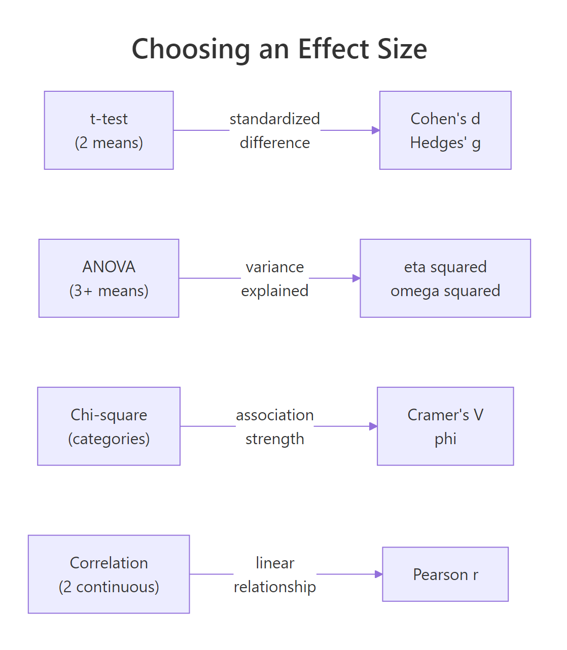
Which effect size family matches each kind of statistical test.

Figure 1: Which effect size family matches each kind of statistical test.

Once you have picked a family, interpretation uses Cohen's benchmarks from his 1988 textbook. They are not laws of nature, but they are widely accepted, and journals expect them as a baseline.

Measure	Small	Medium	Large	Use when
Cohen's d, Hedges' g	0.2	0.5	0.8	Comparing two group means
η², ω²	0.01	0.06	0.14	One-way ANOVA, 3+ groups
Cramér's V (df = 1)	0.10	0.30	0.50	Chi-square, 2×2 or df=1
Pearson's r	0.10	0.30	0.50	Two continuous variables

A tiny helper function turns raw d values into Cohen's labels.

RInterpret Cohen's d against benchmarks

interpret_d <- function(d) { absd <- abs(d) if (absd < 0.2) "negligible" else if (absd < 0.5) "small" else if (absd < 0.8) "medium" else "large" } # Apply to the d values we computed earlier c(d_mpg = interpret_d(d_mpg), d_bigN = interpret_d(d_bigN)) #> d_mpg d_bigN #> "large" "negligible"

The mtcars d of 1.48 lands firmly in "large," while the 20000-observation simulation d of 0.05 is "negligible" despite its tiny p-value. Same interpretive framework, opposite substantive conclusions.

Note

Cohen's benchmarks are guidelines, not laws. A d of 0.2 in a cancer trial can save thousands of lives; a d of 1.0 in a marketing A/B test may be field-trivial if the baseline conversion is already 0.1 percent. Always interpret in domain context.

Tip

Report effect size with a confidence interval when possible. A point estimate of d = 0.45 with 95% CI [0.05, 0.85] is far less conclusive than d = 0.45 with CI [0.40, 0.50]. Modern methods, including bootstrap, can attach CIs to any of the effect sizes shown here.

Try it: You analyzed survey responses from 500 people and found that a new training program correlates with test-score improvement at r = 0.42. Classify this effect size.

RYour turn: classify an effect size

ex_r_train <- 0.42 # your code here # Expected output: "large" (r >= 0.5 is large, 0.3-0.5 is medium)

Click to reveal solution

RClassify r solution

interpret_r <- function(r) { absr <- abs(r) if (absr < 0.10) "negligible" else if (absr < 0.30) "small" else if (absr < 0.50) "medium" else "large" } interpret_r(ex_r_train) #> [1] "medium"

Explanation: r = 0.42 falls in the 0.30–0.50 range, making it a "medium" effect under Cohen's benchmarks for correlations. Worth acting on, but not a ceiling effect.

Practice Exercises

Exercise 1: Report η² for iris

Run a one-way ANOVA of Petal.Length explained by Species in the iris dataset. Extract F, the p-value, and compute η² and ω². Save the three numbers in a named vector called my_iris_report.

RExercise 1: iris ANOVA with effect size

# Write your code below

Click to reveal solution

RExercise 1 solution

my_fit <- aov(Petal.Length ~ Species, data = iris) my_atbl <- summary(my_fit)[[1]] my_F <- my_atbl$"F value"[1] my_p <- my_atbl$"Pr(>F)"[1] my_ss_b <- my_atbl$"Sum Sq"[1] my_ss_t <- sum(my_atbl$"Sum Sq") my_df_b <- my_atbl$Df[1] my_ms_err <- my_atbl$"Mean Sq"[2] my_eta <- my_ss_b / my_ss_t my_omega <- (my_ss_b - my_df_b * my_ms_err) / (my_ss_t + my_ms_err) my_iris_report <- round(c(F = my_F, p = my_p, eta2 = my_eta, omega2 = my_omega), 4) print(my_iris_report) #> F p eta2 omega2 #> 1180.16 0.0000 0.9414 0.9410

Explanation: Species explains about 94 percent of the variance in petal length, one of the largest ANOVA effects you will ever see. η² and ω² agree closely because the sample is large (n = 150).

Exercise 2: Ozone in May vs August

Compare May and August ozone readings in the airquality dataset. Drop NA rows with na.omit() first. Run Welch's t-test, then compute Cohen's d and Hedges' g using the functions from earlier. Interpret d against Cohen's benchmarks.

RExercise 2: airquality effect size

# Hint: filter Ozone by Month == 5 and Month == 8, drop NAs # Use cohens_d() and hedges_g() defined earlier

Click to reveal solution

RExercise 2 solution

my_may <- na.omit(airquality$Ozone[airquality$Month == 5]) my_aug <- na.omit(airquality$Ozone[airquality$Month == 8]) my_t <- t.test(my_aug, my_may) my_d <- cohens_d(my_aug, my_may) my_g <- hedges_g(my_aug, my_may) round(c( p = my_t$p.value, d = my_d, g = my_g ), 3) #> p d g #> 0.000 1.343 1.321

Explanation: August ozone averages about 1.34 pooled SDs above May, which is a very large effect. Hedges' g is only 0.02 lower because the combined sample is healthy. Interpretation: the seasonal effect on ozone is large, not just "statistically detectable."

Complete Example: Effect size report for mtcars

A full effect-size report usually pairs each test in your analysis with its matching effect size. Here is that workflow end-to-end on mtcars, touching all four families covered above.

RComplete example: four effect sizes on mtcars

# 1. Cohen's d: mpg by transmission (2 groups) mt_d <- cohens_d(manual, auto) # 2. eta-squared: mpg by cylinder (3 groups, ANOVA) mt_fit <- aov(mpg ~ factor(cyl), data = mtcars) mt_atbl <- summary(mt_fit)[[1]] mt_eta <- mt_atbl$"Sum Sq"[1] / sum(mt_atbl$"Sum Sq") # 3. Cramer's V: gear by cyl (categorical association) mt_tab <- table(mtcars$gear, mtcars$cyl) mt_chi <- suppressWarnings(chisq.test(mt_tab)) mt_v <- sqrt(as.numeric(mt_chi$statistic) / (sum(mt_tab) * (min(dim(mt_tab)) - 1))) # 4. Pearson r: mpg by weight (continuous pair) mt_r <- cor(mtcars$mpg, mtcars$wt) round(c( "Cohen d (mpg ~ am)" = mt_d, "eta2 (mpg ~ cyl)" = mt_eta, "Cramer V (gear ~ cyl)" = mt_v, "Pearson r (mpg ~ wt)" = mt_r ), 3) #> Cohen d (mpg ~ am) eta2 (mpg ~ cyl) Cramer V (gear ~ cyl) #> 1.478 0.732 0.637 #> Pearson r (mpg ~ wt) #> -0.868

Reading the output: transmission type, cylinder count, gear-cylinder association, and vehicle weight all have very large relationships with mpg. Every number sits above Cohen's "large" cutoff. That is expected for mtcars because it was assembled to contrast very different car designs, not to look like real-world sampling noise.

In a real report, you would pair each number with its test statistic and p-value. The effect size is the punchline, but the test confirms it is not a sampling fluke.

Summary

Effect size is the number that turns "the groups differ" into "here is how much they differ, on a scale I can interpret." Use the right family for your data structure, interpret against Cohen's benchmarks while accounting for your domain, and you will never again read a p-value as a magnitude.

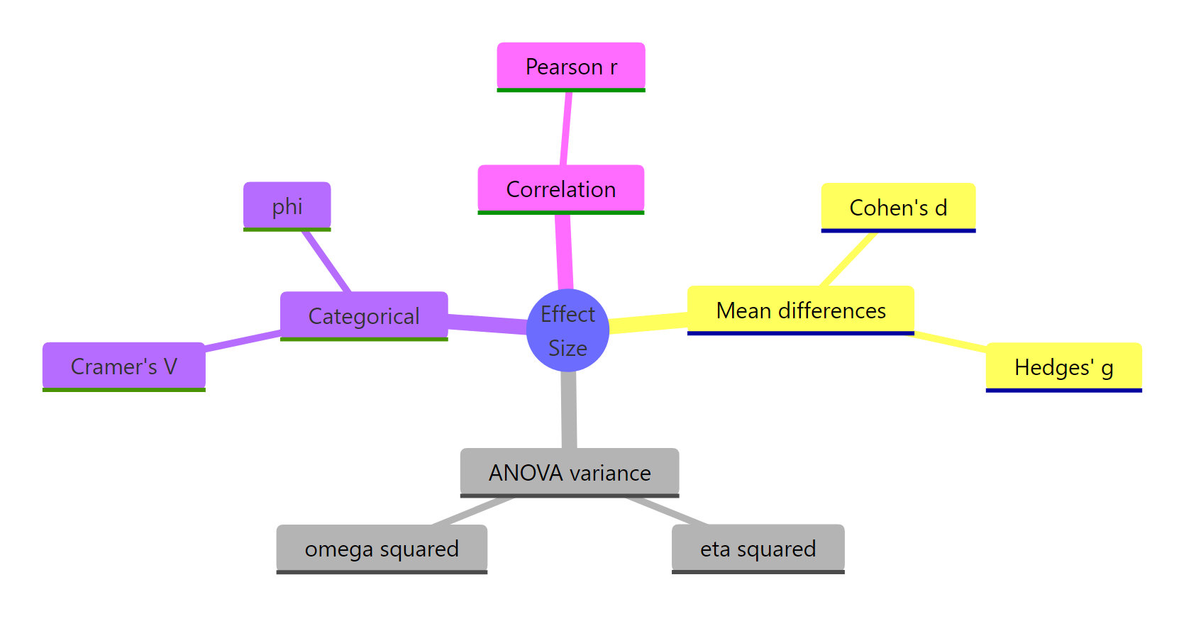
Families of effect size and their key members.

Figure 2: Families of effect size and their key members.

Question	Measure	Small / Medium / Large	Base-R recipe
Do two groups differ?	Cohen's d, Hedges' g	0.2 / 0.5 / 0.8	Mean diff / pooled SD
Does a factor explain variance?	η², ω²	0.01 / 0.06 / 0.14	SS_between / SS_total
Are two categories associated?	Cramér's V, phi	0.10 / 0.30 / 0.50 (df=1)	√(χ² / (N·(k−1)))
Do two continuous variables relate?	Pearson r, r²	0.10 / 0.30 / 0.50	`cor(x, y)`

Three habits go with the table. Always report effect size when you report a p-value. Always note your benchmark source (Cohen, Sawilowsky, or a domain-specific paper). Always attach a confidence interval if your sample is small enough that the point estimate could shift meaningfully with more data.

References

Cohen, J. Statistical Power Analysis for the Behavioral Sciences, 2nd ed. Lawrence Erlbaum (1988). Link
Lakens, D. (2013). Calculating and reporting effect sizes to facilitate cumulative science: a practical primer for t-tests and ANOVAs. Frontiers in Psychology, 4, 863. Link
Cumming, G. (2014). The New Statistics: Why and How. Psychological Science, 25(1), 7–29. Link
Nakagawa, S. & Cuthill, I. C. (2007). Effect size, confidence interval and statistical significance: a practical guide for biologists. Biological Reviews, 82, 591–605. Link
Olejnik, S. & Algina, J. (2003). Generalized eta and omega squared statistics: measures of effect size for some common research designs. Psychological Methods, 8(4), 434–447. Link
American Psychological Association (2020). Publication Manual of the American Psychological Association, 7th ed. Link
R Core Team. An Introduction to R, base R documentation for aov(), chisq.test(), cor(). Link

Continue Learning

Hypothesis Testing in R: runs the tests whose effect sizes this post computes, from two-sample t-tests to chi-square.
Power Analysis in R: feed your planned effect size into power analysis to get the sample size your study needs. Closes the design loop.
Measures of Association in R: deeper coverage of categorical association measures beyond Cramér's V, including Kendall's tau-b and Goodman-Kruskal's gamma.

Effect Size in R: The Number p-Values Never Tell You (Cohen's d, η², and r)

Why does effect size matter more than p-values?

How do you compute Cohen's d for two groups in R?

How do you measure effect size for ANOVA (η² and ω²)?

What effect size do you use for categorical variables (Cramér's V)?

How do you interpret Pearson's r as an effect size?

Which effect size should you use?

Practice Exercises

Exercise 1: Report η² for iris

Exercise 2: Ozone in May vs August

Complete Example: Effect size report for mtcars

Summary

References

Continue Learning

Related Tutorials