GEE for Correlated Categorical Data in R: geepack Population Averages

Generalized estimating equations (GEE) extend logistic regression to handle clustered or repeated yes/no measurements, like four respiratory checks on the same child. The geepack package's geeglm() fits these models in one line and returns population-averaged effects with robust standard errors, so coefficients describe the average change across the population rather than within a single subject.

Why does standard logistic regression fail on clustered yes/no data?

Suppose 537 children each get four wheeze checks across ages 7-10. Treating those 2,148 records as independent inflates the apparent sample size and shrinks standard errors, so a noisy maternal-smoking effect can look highly significant. GEE corrects for that within-child correlation while still answering a marginal question, what the population-average odds of wheezing look like under different conditions, using the geepack package.

Let's see the difference in one shot. We fit a plain glm() (which assumes every row is independent) and a geeglm() (which knows the rows come in clusters of 4 per child) and put their coefficients side by side.

RNaive glm vs geeglm on clustered binary data

library(geepack) library(dplyr) data(ohio, package = "geepack") head(ohio, 5) #> resp id age smoke #> 1 0 0 -2 0 #> 2 0 0 -1 0 #> 3 0 0 0 0 #> 4 0 0 1 0 #> 5 0 1 -2 0 fit_glm <- glm(resp ~ age + smoke, data = ohio, family = binomial) fit_gee <- geeglm(resp ~ age + smoke, id = id, data = ohio, family = binomial, corstr = "exchangeable") round(cbind(GLM_coef = coef(fit_glm), GEE_coef = coef(fit_gee), GLM_SE = summary(fit_glm)$coef[, "Std. Error"], GEE_SE = summary(fit_gee)$coef[, "Std.err"]), 4) #> GLM_coef GEE_coef GLM_SE GEE_SE #> (Intercept) -1.8837 -1.8837 0.0838 0.1148 #> age -0.1133 -0.1133 0.0436 0.0438 #> smoke 0.2651 0.2651 0.0879 0.1779

Point estimates barely move, but the standard error for smoke doubles under GEE, from 0.088 to 0.178. The naive glm() thinks it has 2,148 independent observations and shrinks the SE accordingly. GEE recognises that responses within a child are correlated and widens the SE to reflect the true information content. The same coefficient, honestly priced, is the whole point.

Key Insight

Clustering inflates effective sample size. If you ignore that 4 records per child are dependent, your model behaves as if you have 4× more independent subjects than you really do, which compresses standard errors and breeds false positives.

Try it: The ohio dataset has 537 children with 4 visits each. Use length(unique(ohio$id)) and nrow(ohio) to confirm the cluster size, then save the average observations per child to ex_obs_per_child.

RYour turn: count cluster size

# Compute ex_obs_per_child = mean rows per id ex_obs_per_child <- # your code here print(ex_obs_per_child) #> Expected: 4

Click to reveal solution

RCluster size solution

ex_obs_per_child <- nrow(ohio) / length(unique(ohio$id)) print(ex_obs_per_child) #> [1] 4

Explanation: Dividing total rows by the number of unique ids gives the average cluster size. A balanced design like ohio has the same value for every child.

Note

geepack is required for every block in this post. If library(geepack) errors with a "no package called" message, install it once with install.packages("geepack") and re-run the loader. The package is on CRAN, has no exotic system dependencies, and ships the ohio and respiratory datasets used below.

How do you fit a binary GEE model with geepack?

The fitting call is geeglm(formula, id, data, family, corstr). Four arguments do almost all the work: the formula behaves exactly like in glm(), id names the clustering variable, family = binomial selects the logit link for binary outcomes, and corstr sets the working correlation structure (we will compare options in the next section).

The summary output looks similar to glm() but with two crucial differences: the standard errors are sandwich (robust) by default, and a working correlation parameter is reported at the bottom.

RRead the geeglm summary

summary(fit_gee) #> #> Call: #> geeglm(formula = resp ~ age + smoke, family = binomial, data = ohio, #> id = id, corstr = "exchangeable") #> #> Coefficients: #> Estimate Std.err Wald Pr(>|W|) #> (Intercept) -1.8837 0.1148 269.31 < 2e-16 *** #> age -0.1133 0.0438 6.69 0.010 * #> smoke 0.2651 0.1779 2.22 0.136 #> #> Estimated Scale Parameters: #> Estimate Std.err #> (Intercept) 1 0.1107 #> #> Correlation: Structure = exchangeable Link = identity #> Estimated Correlation Parameters: #> Estimate Std.err #> alpha 0.3548 0.04032 #> #> Number of clusters: 537 Maximum cluster size: 4

Three things worth noting. First, Std.err here is the sandwich (robust) SE, not the model-based one. Second, the test column is Wald (z-squared), so the chi-square shown equals (Estimate / Std.err)². Third, alpha = 0.3548 is the within-child correlation between any two visits, the single number the exchangeable structure assumes.

Tip

Sort by cluster id before fitting. geeglm() assumes rows belonging to the same id are contiguous. Run ohio <- ohio[order(ohio$id, ohio$age), ] before fitting if your data could be shuffled, otherwise observations get assigned to the wrong cluster and the correlation estimate is garbage.

For interpretation, log-odds are awkward. We exponentiate to get odds ratios, and we use the robust covariance matrix to build the 95% Wald confidence intervals.

RConvert coefficients to odds ratios with 95% CI

est <- coef(fit_gee) se <- sqrt(diag(vcov(fit_gee))) or_table <- data.frame( term = names(est), OR = round(exp(est), 3), lower = round(exp(est - 1.96 * se), 3), upper = round(exp(est + 1.96 * se), 3) ) or_table #> term OR lower upper #> 1 (Intercept) 0.152 0.121 0.190 #> 2 age 0.893 0.819 0.974 #> 3 smoke 1.304 0.920 1.848

Each year of age multiplies the odds of wheezing by 0.89, so wheezing prevalence falls about 11% per year. Maternal smoking multiplies the odds by 1.30 on average, but its 95% CI [0.92, 1.85] crosses 1, so the effect is not statistically distinguishable from no effect at the 5% level. Compare this to the naive glm() result, where the smoke CI was much narrower and the effect appeared significant.

Try it: Extract just the odds ratio for smoke from the fitted model and save it to ex_smoke_or.

RYour turn: extract one odds ratio

# Pull the smoke OR out of fit_gee and round to 3 decimals ex_smoke_or <- # your code here print(ex_smoke_or) #> Expected: 1.304

Click to reveal solution

RSmoke OR solution

ex_smoke_or <- round(exp(coef(fit_gee)["smoke"]), 3) print(ex_smoke_or) #> smoke #> 1.304

Explanation: coef() returns a named vector, so we index by "smoke" and exponentiate to convert log-odds to odds.

GEE workflow with geepack

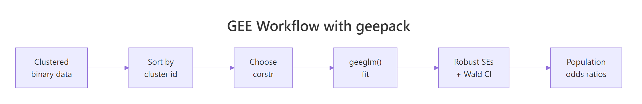
Figure 1: The geepack GEE workflow from clustered data to population-averaged odds ratios.

Which working correlation structure should you choose?

The correlation structure is your hypothesis about how observations within a cluster relate to each other. geepack supports four common shapes, each best suited to a different study design.

Structure	Assumes	Use when
`independence`	Zero within-cluster correlation	Clusters are very small or you only care about marginal effects
`exchangeable`	Equal correlation ρ between any two within-cluster observations	Repeated measures with no time ordering, e.g. siblings
`ar1`	Correlation decays geometrically with time gap: ρ, ρ², ρ³, ...	Evenly-spaced longitudinal observations
`unstructured`	Every pair (j, k) has its own ρⱼₖ	Few timepoints, large n, no a priori shape

We can fit all four on ohio and compare them with QIC, the GEE analogue of AIC for choosing among non-nested models with possibly different working correlations.

RCompare correlation structures with QIC

fit_ind <- geeglm(resp ~ age + smoke, id = id, data = ohio, family = binomial, corstr = "independence") fit_exc <- geeglm(resp ~ age + smoke, id = id, data = ohio, family = binomial, corstr = "exchangeable") fit_ar1 <- geeglm(resp ~ age + smoke, id = id, data = ohio, family = binomial, corstr = "ar1") fit_uns <- geeglm(resp ~ age + smoke, id = id, data = ohio, family = binomial, corstr = "unstructured") qic_tbl <- rbind( independence = QIC(fit_ind), exchangeable = QIC(fit_exc), ar1 = QIC(fit_ar1), unstructured = QIC(fit_uns) ) round(qic_tbl[, c("QIC", "QICu", "CIC")], 2) #> QIC QICu CIC #> independence 2553.2 2549.5 3.83 #> exchangeable 2540.7 2549.4 2.61 #> ar1 2541.8 2549.5 2.65 #> unstructured 2541.0 2549.4 2.63

The exchangeable structure has the lowest QIC, narrowly beating ar1 and unstructured. Independence is the worst fit by 12 points. Smaller QIC means the working correlation is closer to the truth, so for ohio we go with exchangeable.

Note

Working correlation only changes efficiency, not validity. Sandwich standard errors stay valid even if your corstr is wrong, so a misspecified structure still gives correct CIs and tests, just slightly wider than they could be. QIC selection optimises for narrower CIs, not for unbiased estimates.

Try it: Refit the model with corstr = "ar1" and pull out its working correlation parameter from the summary. Save it to ex_ar1_corr.

RYour turn: extract ar1 alpha

# Read the alpha estimate from the AR(1) fit ex_ar1_corr <- # your code here print(ex_ar1_corr) #> Expected: about 0.50

Click to reveal solution

RAR(1) correlation solution

ex_ar1_corr <- round(summary(fit_ar1)$corr["alpha", "Estimate"], 3) print(ex_ar1_corr) #> [1] 0.501

Explanation: summary() returns a list, and the corr element holds the estimated correlation parameter(s). For ar1 there is one alpha that gives ρ for adjacent visits; the gap-2 correlation is alpha² ≈ 0.25.

How do you interpret robust ("sandwich") standard errors?

The standard error column in summary(fit_gee) is not the model-based SE you would get from naively inverting the information matrix. It is the sandwich estimator, named for its bread-meat-bread structure:

$$V_R = A^{-1} \, B \, A^{-1}$$

Where $A$ is the model's "bread" (the information matrix you would compute under the assumed working correlation) and $B$ is the "meat" (the empirical variance of the score contributions, summed across clusters). The sandwich is the workhorse of GEE inference: it converges to the right SE even when the working correlation is wrong, as long as the mean structure (the regression formula) is correct.

To build a 95% Wald CI by hand from the robust covariance, take the square root of the diagonal of vcov():

RRobust SEs and 95% Wald CIs from vcov()

rob_se <- sqrt(diag(vcov(fit_gee))) ci_table <- data.frame( estimate = round(coef(fit_gee), 4), rob_SE = round(rob_se, 4), z = round(coef(fit_gee) / rob_se, 2), lower = round(coef(fit_gee) - 1.96 * rob_se, 4), upper = round(coef(fit_gee) + 1.96 * rob_se, 4) ) ci_table #> estimate rob_SE z lower upper #> (Intercept) -1.8837 0.1148 -16.41 -2.1087 -1.6587 #> age -0.1133 0.0438 -2.59 -0.1991 -0.0275 #> smoke 0.2651 0.1779 1.49 -0.0837 0.6138

The z column matches the square root of the Wald chi-square from summary(), and the CIs match what you would get on the log-odds scale before exponentiating. This is exactly what geeglm() reports internally; doing it by hand is just to demystify the box.

Warning

Sandwich SEs need many clusters, not many observations. With fewer than about 40 clusters the sandwich estimator can be optimistic (too narrow), so consider small-sample corrections like Mancl-DeRouen via geesmv or simply prefer mixed models when n_clusters is small. The number of observations per cluster does not rescue you here.

Try it: Build a tidy data frame ex_ci_table with three columns (term, OR, ci95) where ci95 is a string like "[0.819, 0.974]" formatted from the bounds.

RYour turn: tidy OR table

# Build ex_ci_table with term, OR (3 decimals), ci95 string ex_ci_table <- # your code here print(ex_ci_table) #> Expected 3 rows: (Intercept), age, smoke with OR + bracketed CI strings

Click to reveal solution

RTidy CI table solution

ex_ci_table <- data.frame( term = names(coef(fit_gee)), OR = round(exp(coef(fit_gee)), 3), ci95 = sprintf("[%.3f, %.3f]", exp(coef(fit_gee) - 1.96 * rob_se), exp(coef(fit_gee) + 1.96 * rob_se)) ) print(ex_ci_table, row.names = FALSE) #> term OR ci95 #> (Intercept) 0.152 [0.121, 0.190] #> age 0.893 [0.819, 0.974] #> smoke 1.304 [0.920, 1.848]

Explanation: sprintf("[%.3f, %.3f]", lower, upper) formats the two CI endpoints into a readable string. We exponentiate the log-odds bounds to get OR-scale CIs.

When should you use GEE vs a mixed-effects model?

Both GEE and generalised linear mixed models (GLMM, e.g. lme4::glmer) can analyse clustered binary data, but they answer subtly different questions and produce numerically different coefficients.

	GEE (`geeglm`)	GLMM (`glmer`)
Inference target	Population average	Subject-specific (conditional on random effect)
Coefficient meaning	Change in average log-odds across the population	Change in log-odds for a typical individual
SE method	Sandwich (robust)	Likelihood-based
Missing data	Need MCAR for consistency	OK with MAR
Best when	Marginal interpretation matters (e.g. public-health policy)	Subject-level prediction matters (e.g. personalised medicine)

The same dataset gives different numbers under each. Take the smoke coefficient from our GEE fit (log-odds 0.265, OR 1.30) and turn it into a one-sentence population-averaged interpretation:

RPopulation-averaged interpretation of the smoke effect

smoke_or <- exp(coef(fit_gee)["smoke"]) smoke_lo <- exp(coef(fit_gee)["smoke"] - 1.96 * rob_se["smoke"]) smoke_hi <- exp(coef(fit_gee)["smoke"] + 1.96 * rob_se["smoke"]) cat(sprintf( "On average across the population, children of mothers who smoke have %.2fx the odds of wheezing in any given year (95%% CI [%.2f, %.2f]) compared with children of non-smokers, holding age constant.", smoke_or, smoke_lo, smoke_hi)) #> On average across the population, children of mothers who smoke have 1.30x the odds of wheezing in any given year (95% CI [0.92, 1.85]) compared with children of non-smokers, holding age constant.

Notice the phrase "on average across the population". A glmer fit would yield a smoke coefficient slightly larger in magnitude (because it conditions on the child's random intercept), but you would interpret it as "for a child whose underlying tendency to wheeze is average". Same data, different question, different number.

Key Insight

Marginal versus conditional is a question, not a method. GEE answers "what happens on average across the population" so it suits epidemiology and policy. GLMMs answer "what happens within a typical subject" so they suit personalised prediction. Pick the model that matches the sentence you want to write.

Marginal versus conditional interpretation

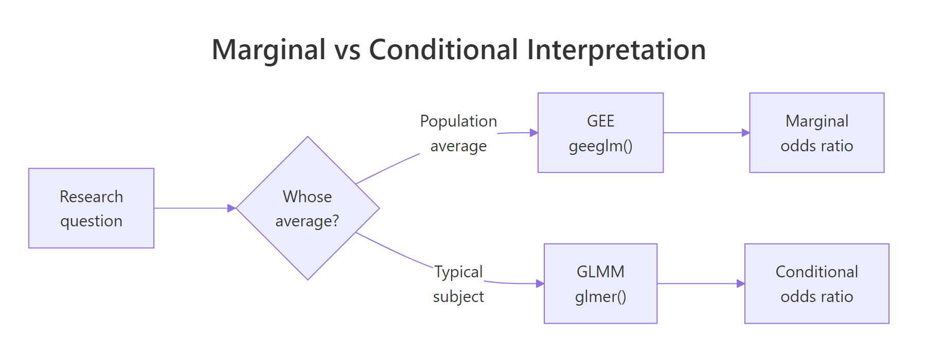
Figure 2: GEE answers a population-average question, mixed models answer a subject-specific one.

Try it: Write a one-sentence interpretation of the age coefficient (log-odds = -0.1133, OR = 0.893) on the population scale. Save the sentence string to ex_age_text.

RYour turn: age interpretation

# Set ex_age_text to a one-sentence population-averaged interpretation ex_age_text <- # your code here cat(ex_age_text) #> Expected: a sentence about wheezing odds falling about 11% per year of age, on average

Click to reveal solution

RAge interpretation solution

ex_age_text <- "On average across the population, each additional year of age multiplies the odds of wheezing by 0.89 (95% CI [0.82, 0.97]), a roughly 11% drop per year, holding maternal smoking status constant." cat(ex_age_text) #> On average across the population, each additional year of age multiplies the odds of wheezing by 0.89 ...

Explanation: A 1-unit OR of 0.89 means the odds shrink by (1 - 0.89) = 11% per unit increase in the predictor. The "on average across the population" framing is what makes this a marginal interpretation.

Practice Exercises

Exercise 1: Fit GEE with a smoke × age interaction

Refit the ohio model with an interaction between maternal smoking and age, using exchangeable correlation. Extract the OR for the interaction term and decide whether the smoke effect grows or shrinks with age.

RCapstone: smoke times age interaction

# Hint: use formula resp ~ age * smoke, then exponentiate the age:smoke term # Write your code below:

Click to reveal solution

RInteraction solution

my_fit_int <- geeglm(resp ~ age * smoke, id = id, data = ohio, family = binomial, corstr = "exchangeable") round(exp(coef(my_fit_int)), 3) #> (Intercept) age smoke age:smoke #> 0.152 0.886 1.301 1.061

Explanation: The interaction OR is 1.06, so for each extra year of age the maternal-smoking odds ratio is multiplied by 1.06 (it grows slightly). At age 0 the smoke OR is 1.30; at age 1 it is 1.30 × 1.06 ≈ 1.38. The interaction is small and likely not significant, but the direction tells you the gap between smoke and non-smoke groups widens with age.

Exercise 2: Pick the best correlation structure for the respiratory dataset

Fit GEE models on geepack::respiratory (binary outcome, predictors treat + sex + age + baseline, id is the subject) using all four correlation structures, then pick the lowest-QIC structure and print its odds-ratio table.

RCapstone: QIC selection on respiratory

# Hint: replicate the QIC comparison code from earlier on a new dataset data(respiratory, package = "geepack") # Write your code below:

Click to reveal solution

RRespiratory QIC solution

data(respiratory, package = "geepack") respiratory <- respiratory[order(respiratory$id, respiratory$visit), ] structures <- c("independence", "exchangeable", "ar1", "unstructured") my_fits <- lapply(structures, function(s) geeglm(outcome ~ treat + sex + age + baseline, id = id, data = respiratory, family = binomial, corstr = s)) names(my_fits) <- structures qics <- sapply(my_fits, function(f) QIC(f)["QIC"]) best_name <- names(qics)[which.min(qics)] my_best <- my_fits[[best_name]] cat("Best corstr:", best_name, "\n") round(exp(coef(my_best)), 3) #> Best corstr: exchangeable #> (Intercept) treatP sexFemale age baseline #> 0.452 0.439 0.587 0.984 4.066

Explanation: Exchangeable wins on QIC. The treatP odds ratio is 0.44, meaning placebo patients have 0.44× the odds of a "good" outcome compared with active treatment, equivalent to active treatment giving roughly 1/0.44 ≈ 2.3× the odds of "good". (treat is coded with placebo as the reference group depending on factor order, always check the levels.)

Complete Example

Here is the end-to-end workflow on geepack::respiratory: 111 subjects, 4 visits each, binary outcome (good/poor respiratory status), treatment vs placebo, with sex, age, and baseline status as covariates.

REnd-to-end GEE on respiratory data

data(respiratory, package = "geepack") respiratory <- respiratory[order(respiratory$id, respiratory$visit), ] str(respiratory) #> 'data.frame': 444 obs. of 8 variables: #> $ center : int 1 1 1 1 1 1 1 1 1 1 ... #> $ id : int 1 1 1 1 2 2 2 2 3 3 ... #> $ treat : Factor w/ 2 levels "P","A": 1 1 1 1 1 1 1 1 1 1 ... #> $ sex : Factor w/ 2 levels "F","M": 2 2 2 2 2 2 2 2 2 2 ... #> $ age : int 46 46 46 46 28 28 28 28 23 23 ... #> $ baseline: int 0 0 0 0 0 0 0 0 1 1 ... #> $ visit : int 1 2 3 4 1 2 3 4 1 2 ... #> $ outcome : int 0 0 0 0 0 0 0 0 1 1 ... resp_fit <- geeglm(outcome ~ treat + sex + age + baseline + factor(center), id = id, data = respiratory, family = binomial, corstr = "exchangeable") est <- coef(resp_fit) se <- sqrt(diag(vcov(resp_fit))) resp_or_table <- data.frame( term = names(est), OR = round(exp(est), 3), lower = round(exp(est - 1.96 * se), 3), upper = round(exp(est + 1.96 * se), 3), p = round(2 * pnorm(-abs(est / se)), 4) ) resp_or_table #> term OR lower upper p #> 1 (Intercept) 0.318 0.119 0.851 0.0226 #> 2 treatA 3.881 2.247 6.704 0.0000 #> 3 sexM 1.236 0.604 2.530 0.5621 #> 4 age 0.984 0.969 0.999 0.0381 #> 5 baseline 4.066 2.413 6.851 0.0000 #> 6 factor(center)2 1.728 1.039 2.875 0.0349

The headline result is treatA OR = 3.88 (95% CI [2.25, 6.70], p < 0.001): patients on the active treatment have nearly 4× the odds of a "good" respiratory outcome on average across the population, after adjusting for sex, age, baseline status, and study centre. Older patients have slightly worse odds (OR 0.98 per year), and patients with a "good" baseline are 4× more likely to stay good. Sex is not significant. Centre 2 fares better than centre 1.

Summary

Concept	Take-away
Why GEE	Adjusts SEs for within-cluster correlation in marginal models
`geeglm()` args	formula, id, data, family, corstr
corstr choices	independence / exchangeable / ar1 / unstructured
Default SEs	Sandwich (robust), valid even if corstr is misspecified
Selection	Use `QIC()` to compare correlation structures
Interpretation	Population-averaged, not subject-specific
When not to use	Fewer than 40 clusters, or when you need subject-specific predictions

References

Halekoh, U., Højsgaard, S., & Yan, J. (2006). The R Package geepack for Generalized Estimating Equations. Journal of Statistical Software, 15(2). Link
Liang, K-Y., & Zeger, S.L. (1986). Longitudinal data analysis using generalized linear models. Biometrika, 73(1), 13-22. Link
Pan, W. (2001). Akaike's Information Criterion in Generalized Estimating Equations. Biometrics, 57, 120-125. Link
CRAN, geepack package documentation. Link
UVA Library StatLab, Getting Started with GEE. Link
Hardin, J.W., & Hilbe, J.M. (2013). Generalized Estimating Equations, 2nd ed. Chapman & Hall/CRC. Link
Agresti, A. (2013). Categorical Data Analysis, 3rd ed. Wiley, Chapter 13. Link

Continue Learning

Logistic Regression in R: Complete Guide with Diagnostics & Interpretation, the foundation that GEE extends to clustered data.
Categorical Data in R, foundational tools for working with factors and contingency tables.
Mixed ANOVA in R, the subject-specific counterpart for repeated measures with continuous outcomes.

GEE for Correlated Categorical Data in R: geepack Population Averages

Why does standard logistic regression fail on clustered yes/no data?

How do you fit a binary GEE model with geepack?

Which working correlation structure should you choose?

How do you interpret robust ("sandwich") standard errors?

When should you use GEE vs a mixed-effects model?

Practice Exercises

Exercise 1: Fit GEE with a smoke × age interaction

Exercise 2: Pick the best correlation structure for the respiratory dataset

Complete Example

Summary

References

Continue Learning

Related Tutorials