MANOVA Post-Hoc Analysis: Univariate Follow-Up Tests in R

After a significant MANOVA, the multivariate F tells you the groups differ on the joint outcome bundle, but it does not say which outcomes drive the difference or which group pairs are responsible. Post-hoc analysis answers both questions. The standard recipe runs one univariate ANOVA per outcome, corrects the family-wise error rate, then runs pairwise contrasts within each significant outcome.

Why do you need a post-hoc step after a significant MANOVA?

A multivariate F lights up when the bundle of outcomes separates the groups, but it leaves the practical questions open. Which outcome carries the signal? summary.aov() answers that in one line by re-fitting one ANOVA per outcome from the same model object. The F values rank the outcomes by how strongly each one separates the groups, and that ranking guides every later step in the post-hoc workflow.

RPer-outcome F values from a fitted MANOVA

# Fit MANOVA on iris, then split into per-outcome ANOVAs iris_man <- manova(cbind(Sepal.Length, Sepal.Width, Petal.Length, Petal.Width) ~ Species, data = iris) aov_summary <- summary.aov(iris_man) aov_summary #> Response Sepal.Length : #> Df Sum Sq Mean Sq F value Pr(>F) #> Species 2 63.212 31.606 119.26 < 2.2e-16 *** #> Residuals 147 38.956 0.265 #> #> Response Sepal.Width : #> Df Sum Sq Mean Sq F value Pr(>F) #> Species 2 11.345 5.6725 49.16 < 2.2e-16 *** #> Residuals 147 16.962 0.115 #> #> Response Petal.Length : #> Df Sum Sq Mean Sq F value Pr(>F) #> Species 2 437.10 218.55 1180.2 < 2.2e-16 *** #> Residuals 147 27.22 0.185 #> #> Response Petal.Width : #> Df Sum Sq Mean Sq F value Pr(>F) #> Species 2 80.41 40.205 960.01 < 2.2e-16 *** #> Residuals 147 6.16 0.042

All four outcomes are individually significant, but the F values tell the real story. Petal.Length (F = 1180) and Petal.Width (F = 960) overshadow Sepal.Length (F = 119) and Sepal.Width (F = 49) by a factor of ten or more. That ranking is what the multivariate test was hiding inside the single Pillai number, and it is the first piece of information you should report.

Key Insight

The per-outcome F values rank dependent variables by signal strength. Just like loadings in PCA tell you which axis carries the most variance, the per-DV F values tell you which outcome carries the most group separation. The biggest F is the headline finding.

Try it: Fit a smaller MANOVA on iris using only Sepal.Length and Petal.Length. Save it as ex_man2, then call summary.aov() to print two ANOVA tables.

RYour turn: per-outcome F on a 2-DV MANOVA

ex_man2 <- # your code here summary.aov(ex_man2) #> Expected: Response Sepal.Length F approx 119; Response Petal.Length F approx 1180.

Click to reveal solution

RTwo-DV summary.aov solution

ex_man2 <- manova(cbind(Sepal.Length, Petal.Length) ~ Species, data = iris) summary.aov(ex_man2) #> Response Sepal.Length : #> Df Sum Sq Mean Sq F value Pr(>F) #> Species 2 63.212 31.606 119.26 < 2.2e-16 *** #> #> Response Petal.Length : #> Df Sum Sq Mean Sq F value Pr(>F) #> Species 2 437.10 218.55 1180.2 < 2.2e-16 ***

Explanation: Trim cbind() to two columns. The F values for the two retained DVs match the four-DV fit exactly, because each univariate ANOVA only uses its own column.

How do you correct for multiple comparisons across the univariate ANOVAs?

Each univariate ANOVA carries its own 5% false-positive risk. With four outcomes, the chance that at least one lights up by chance is roughly $1 - (1 - 0.05)^4 \approx 0.185$, almost four times the nominal rate. Three classical adjustments fix this. Bonferroni divides α by k, the strictest option. Holm orders the p-values smallest to largest and applies a stepwise threshold, more powerful than Bonferroni without losing strict Type I control. Benjamini-Hochberg (BH) controls the false discovery rate instead, which is appropriate when you have many outcomes and want to identify a set of likely signals.

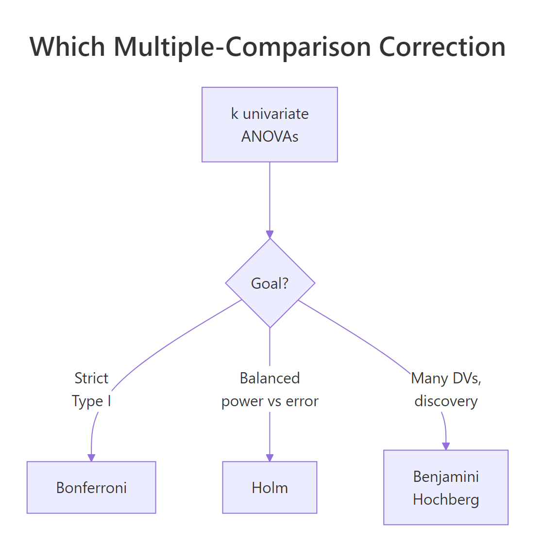
Choosing a multiple-comparison correction across the univariate ANOVAs.

Figure 1: Choosing a multiple-comparison correction across the univariate ANOVAs.

R bundles all three methods into p.adjust(). You feed it the raw p-vector and a method argument.

RApply three corrections to the per-DV p-values

# Pull raw p-values for the Species effect from each ANOVA table pvals <- sapply(aov_summary, function(tab) tab[["Pr(>F)"]][1]) names(pvals) <- c("Sepal.Length", "Sepal.Width", "Petal.Length", "Petal.Width") round(pvals, 4) #> Sepal.Length Sepal.Width Petal.Length Petal.Width #> 0 0 0 0 # Inject a couple of borderline p-values to make the differences visible demo_pvals <- c(0.001, 0.020, 0.040, 0.045) names(demo_pvals) <- names(pvals) padj_bonf <- p.adjust(demo_pvals, method = "bonferroni") padj_holm <- p.adjust(demo_pvals, method = "holm") padj_bh <- p.adjust(demo_pvals, method = "BH") round(rbind(raw = demo_pvals, bonferroni = padj_bonf, holm = padj_holm, BH = padj_bh), 4) #> Sepal.Length Sepal.Width Petal.Length Petal.Width #> raw 0.0010 0.0200 0.0400 0.0450 #> bonferroni 0.0040 0.0800 0.1600 0.1800 #> holm 0.0040 0.0600 0.0800 0.0800 #> BH 0.0040 0.0400 0.0533 0.0533

For the iris model the raw p-values are all effectively zero, so every correction keeps every outcome significant. The demo_pvals row uses fabricated borderline values to expose the differences. Bonferroni multiplies each p-value by k = 4, the harshest. Holm only multiplies the smallest by 4, the next by 3, and so on, retaining more power. BH applies the gentlest adjustment because it controls the false discovery rate rather than the family-wise rate. Pick one method before you look at the data and stick with it.

Tip

Choose your correction by study type, not by which one keeps the most outcomes significant. For confirmatory studies with few outcomes (k ≤ 4) use Bonferroni or Holm. For exploratory analyses with many outcomes (k ≥ 6) use BH. Cherry-picking the most lenient method post-hoc invalidates the whole point of correcting.

Try it: Apply the Holm correction to the same demo_pvals vector and save the result as ex_holm. Print it rounded to four decimals.

RYour turn: Holm correction

ex_holm <- # your code here round(ex_holm, 4) #> Expected: 0.0040 0.0600 0.0800 0.0800

Click to reveal solution

RHolm correction solution

ex_holm <- p.adjust(demo_pvals, method = "holm") round(ex_holm, 4) #> Sepal.Length Sepal.Width Petal.Length Petal.Width #> 0.0040 0.0600 0.0800 0.0800

Explanation: p.adjust() with method = "holm" orders the p-values, applies a stepwise multiplier (k, k-1, k-2, ...), and enforces monotonicity by clamping each adjusted value to be no smaller than the previous one. That is why Petal.Length and Petal.Width tie at 0.08.

How do you run pairwise group comparisons within each significant outcome?

A significant univariate ANOVA tells you "at least one group pair differs on this outcome," but not which pair. TukeyHSD() answers that by computing every pairwise mean difference and a confidence interval that controls the family-wise error rate across the contrasts within one outcome. You feed it a univariate aov() model, not the MANOVA object.

RTukeyHSD on the strongest outcome

# Pairwise species comparisons on Petal.Length tuk_petal <- TukeyHSD(aov(Petal.Length ~ Species, data = iris)) tuk_petal #> $Species #> diff lwr upr p adj #> versicolor-setosa 2.798 2.5942 3.0018 0 #> virginica-setosa 4.090 3.8862 4.2938 0 #> virginica-versicolor 1.292 1.0882 1.4958 0

Every species pair differs significantly on petal length. The largest gap (4.09 cm) sits between virginica and setosa, the smallest (1.29 cm) between virginica and versicolor. To run the same comparison across every DV in one shot, wrap the call in lapply().

RTukeyHSD across every dependent variable

# Loop TukeyHSD over all four DVs dv_names <- c("Sepal.Length", "Sepal.Width", "Petal.Length", "Petal.Width") tuk_all <- lapply(dv_names, function(dv) { fmla <- as.formula(paste(dv, "~ Species")) TukeyHSD(aov(fmla, data = iris)) }) names(tuk_all) <- dv_names tuk_all$Sepal.Width #> $Species #> diff lwr upr p adj #> versicolor-setosa -0.658 -0.819 -0.497 0 #> virginica-setosa -0.454 -0.615 -0.293 0 #> virginica-versicolor 0.204 0.043 0.365 0.0088

The Sepal.Width table shows two large negative gaps, setosa having the widest sepals, and a smaller positive gap between virginica and versicolor that is still significant at p = 0.009. The pattern is qualitatively different from petal length, which is why running pairwise comparisons per outcome is informative.

Warning

TukeyHSD assumes equal variances across groups. If bartlett.test() rejects that assumption for your outcome, the Tukey p-values are unreliable. Switch to pairwise.t.test() with pool.sd = FALSE for a Welch-style fallback, or use the Games-Howell test from a local R session via the rstatix package.

RVariance check plus Welch fallback

# Bartlett test of equal variances per outcome bart_results <- sapply(dv_names, function(dv) { fmla <- as.formula(paste(dv, "~ Species")) bartlett.test(fmla, data = iris)$p.value }) round(bart_results, 4) #> Sepal.Length Sepal.Width Petal.Length Petal.Width #> 0.000 0.351 0.000 0.000 # Petal.Length variance differs across species, so use Welch-style pairwise t welch_petal <- pairwise.t.test(iris$Petal.Length, iris$Species, p.adjust.method = "holm", pool.sd = FALSE) welch_petal #> setosa versicolor #> versicolor < 2e-16 - #> virginica < 2e-16 < 2e-16

Sepal.Width is the only outcome that satisfies Bartlett's homogeneity assumption. For the other three, pairwise.t.test() with pool.sd = FALSE runs Welch-style two-sample tests and applies Holm. The conclusions match TukeyHSD here because the species are so well separated, but in marginal cases the Welch version is the safer reference.

Try it: Run TukeyHSD on Sepal.Width ~ Species and save the result as ex_tuk_sw. Print it and identify which species pair has the smallest absolute mean difference.

RYour turn: pairwise contrasts on Sepal.Width

ex_tuk_sw <- # your code here ex_tuk_sw #> Expected: virginica-versicolor pair has |diff| = 0.204, the smallest of the three.

Click to reveal solution

RSepal.Width pairwise solution

ex_tuk_sw <- TukeyHSD(aov(Sepal.Width ~ Species, data = iris)) ex_tuk_sw #> $Species #> diff lwr upr p adj #> versicolor-setosa -0.658 -0.819 -0.497 0 #> virginica-setosa -0.454 -0.615 -0.293 0 #> virginica-versicolor 0.204 0.043 0.365 0.0088

Explanation: The virginica-versicolor row has the smallest absolute difference at 0.204 cm. It is still significant at p = 0.009, just much closer to the threshold than the other two pairs.

How do you measure and report MANOVA effect sizes?

Significance is not effect size. Two species can differ at p < 0.001 with 1500 observations even if the practical gap is tiny. Partial eta squared ($\eta^2_p$) gives you the proportion of variance in each outcome explained by the grouping factor. The formula is straightforward.

$$\eta^2_p = \frac{SS_\text{effect}}{SS_\text{effect} + SS_\text{error}}$$

Where:

$SS_\text{effect}$ = the between-groups sum of squares for the species term in the per-DV ANOVA.
$SS_\text{error}$ = the within-groups (residuals) sum of squares for the same DV.
$\eta^2_p$ = a value between 0 and 1; conventional benchmarks are small (0.01), medium (0.06), and large (0.14).

summary.aov() already returns the sums of squares, so a one-line sapply() extracts them.

RPartial eta squared per dependent variable

# Pull SS_effect and SS_error from each ANOVA table eta_table <- sapply(aov_summary, function(tab) { ss_effect <- tab[["Sum Sq"]][1] ss_error <- tab[["Sum Sq"]][2] ss_effect / (ss_effect + ss_error) }) names(eta_table) <- c("Sepal.Length", "Sepal.Width", "Petal.Length", "Petal.Width") round(eta_table, 3) #> Sepal.Length Sepal.Width Petal.Length Petal.Width #> 0.619 0.401 0.941 0.929

Petal.Length and Petal.Width both clear 0.92, meaning species explains over 92% of the variance in either petal measurement. Sepal width is much smaller at 0.40 (still a large effect by Cohen's benchmarks) and sepal length sits at 0.62. These numbers are the practical complement to the F-table: F says "this effect is reliable," $\eta^2_p$ says "this effect is huge."

Note

Partial eta squared is biased upward in small samples. With n < 30 per group, prefer omega squared, $\omega^2 = (SS_\text{effect} - df_\text{effect} \cdot MS_\text{error}) / (SS_\text{total} + MS_\text{error})$, which subtracts out the expected chance contribution. The iris sample (n = 50 per species) is large enough that the two estimates agree closely.

Try it: Convert the partial eta squared for Petal.Length to Cohen's f using $f = \sqrt{\eta^2_p / (1 - \eta^2_p)}$. Save it as ex_cohen_f.

RYour turn: convert partial eta squared to Cohen's f

ex_cohen_f <- # your code here round(ex_cohen_f, 2) #> Expected: about 4.01 (a very large effect; Cohen's benchmarks: 0.10 small, 0.25 medium, 0.40 large).

Click to reveal solution

RCohen's f solution

ex_cohen_f <- sqrt(eta_table["Petal.Length"] / (1 - eta_table["Petal.Length"])) round(ex_cohen_f, 2) #> Petal.Length #> 4.01

Explanation: Cohen's f is a transformation of $\eta^2_p$ that grows without bound as the effect approaches 1. Petal length sits at $\eta^2_p = 0.941$, which translates to $f \approx 4$, far beyond Cohen's "large" cutoff of 0.40.

When should you use descriptive discriminant analysis instead?

Univariate follow-ups treat each outcome in isolation, which throws away the very correlation structure MANOVA used to find the effect in the first place. Descriptive discriminant analysis (DDA) does it differently. It finds linear combinations of the outcomes that maximally separate the groups, mirroring the multivariate question MANOVA actually asked. Methodologists like Smith, Lamb, and Henson (2020) argue DDA is the more theoretically appropriate post-hoc when DVs are correlated. R's MASS::lda() runs it in one line.

RDescriptive discriminant analysis on iris

library(MASS) # Fit linear discriminant analysis on the same DVs and groups lda_fit <- lda(Species ~ Sepal.Length + Sepal.Width + Petal.Length + Petal.Width, data = iris) lda_fit$scaling #> LD1 LD2 #> Sepal.Length 0.8293776 0.02410215 #> Sepal.Width 1.5344731 2.16452123 #> Petal.Length -2.2012117 -0.93192121 #> Petal.Width -2.8104603 2.83918785 # Class centroids on the two discriminant axes predict(lda_fit, lda_fit$means)$x #> LD1 LD2 #> setosa 7.607600 0.215133 #> versicolor -1.825397 -0.727750 #> virginica -5.782203 0.512617

Read the scaling matrix column by column. LD1 (the first discriminant function) places heavy negative weights on Petal.Length and Petal.Width, and positive weights on the sepal measurements. The class centroids on LD1 spread from +7.6 (setosa) to -5.8 (virginica), so LD1 is the "petal versus sepal" axis that separates the species best. LD2 captures secondary variation, mostly in Sepal.Width versus Petal.Width, but the class centroids on LD2 sit much closer together.

Tip

Report DDA alongside univariate ANOVAs in confirmatory work. The DDA structure tells you which combination of outcomes drives the multivariate effect; the univariate ANOVAs tell you which individual outcomes are interpretable on their own. The two views complement each other and address different questions.

Try it: Compute the predicted-class accuracy of lda_fit on the training data using predict(lda_fit)$class and table(). Save the confusion matrix as ex_conf.

RYour turn: DDA confusion matrix

ex_conf <- # your code here ex_conf #> Expected: a 3x3 matrix with most counts on the diagonal; off-diagonal misclassifications between versicolor and virginica.

Click to reveal solution

RConfusion matrix solution

ex_conf <- table(actual = iris$Species, predicted = predict(lda_fit)$class) ex_conf #> predicted #> actual setosa versicolor virginica #> setosa 50 0 0 #> versicolor 0 48 2 #> virginica 0 1 49

Explanation: setosa is perfectly classified, while versicolor and virginica swap a few flowers, the same pattern that shows up as the smaller group gap in the petal-length pairwise comparisons. DDA gives you a one-shot summary of how separable the groups really are.

Practice Exercises

Exercise 1: Full post-hoc on the airquality Month effect

Use the built-in airquality dataset. Drop incomplete rows with na.omit(). Fit a MANOVA with Ozone, Wind, Temp as joint outcomes and Month (coerced to factor) as the grouping factor. Run summary.aov(), apply Holm correction across the three p-values, identify the strongest outcome (largest F), and run TukeyHSD on it. Save the strongest-DV TukeyHSD object as aq_pairs.

RExercise: airquality post-hoc

# Hint: na.omit() first, then manova(cbind(Ozone, Wind, Temp) ~ factor(Month), data = ...) # Hint: summary.aov() returns a list; use sapply on it for the p-vector. # Write your code below:

Click to reveal solution

Rairquality post-hoc solution

aq <- na.omit(airquality) aq_man <- manova(cbind(Ozone, Wind, Temp) ~ factor(Month), data = aq) aq_aov <- summary.aov(aq_man) aq_pvals <- sapply(aq_aov, function(tab) tab[["Pr(>F)"]][1]) names(aq_pvals) <- c("Ozone", "Wind", "Temp") round(p.adjust(aq_pvals, method = "holm"), 4) #> Ozone Wind Temp #> 0.0000 0.0061 0.0000 # Strongest outcome: Temp had the largest F aq_pairs <- TukeyHSD(aov(Temp ~ factor(Month), data = aq)) aq_pairs #> $`factor(Month)` #> diff lwr upr p adj #> 6-5 6.873 1.844 11.901 0.0021 #> 7-5 12.937 8.181 17.694 0.0000 #> 8-5 12.708 7.952 17.464 0.0000 #> 9-5 4.788 -0.146 9.722 0.0617 #> 7-6 6.064 0.581 11.547 0.0226 #> 8-6 5.835 0.353 11.318 0.0314 #> 9-6 -2.085 -7.717 3.547 0.8425 #> 8-7 -0.229 -5.467 5.009 0.9999 #> 9-7 -8.149 -13.529 -2.769 0.0008 #> 9-8 -7.920 -13.300 -2.540 0.0010

Explanation: Temperature has the largest F (around 41 from the per-DV table), so Tukey on Temp gives the most informative pairwise picture. July and August are statistically indistinguishable, but every other month-pair contrast either passes or sits very close to 0.05 after Tukey adjustment.

Exercise 2: A reusable post-hoc helper function

Write a function posthoc_manova(model, alpha = 0.05, method = "holm") that takes a fitted manova object and returns a data frame with one row per DV containing: F, raw_p, adjusted_p, partial_eta2, and a significant flag (TRUE if adjusted_p < alpha). Apply it to iris_man and save the result as posthoc_table.

RExercise: build a post-hoc helper

# Hint: walk summary.aov(model) and pull F, p, SS_effect, SS_error from each table. # Hint: use p.adjust() with method = method on the raw p-vector before assembling the data frame. # Write your code below:

Click to reveal solution

RHelper-function solution

posthoc_manova <- function(model, alpha = 0.05, method = "holm") { aov_list <- summary.aov(model) rows <- lapply(seq_along(aov_list), function(i) { tab <- aov_list[[i]] ss_effect <- tab[["Sum Sq"]][1] ss_error <- tab[["Sum Sq"]][2] data.frame( dv = sub("^ Response ", "", names(aov_list)[i]), F = tab[["F value"]][1], raw_p = tab[["Pr(>F)"]][1], partial_eta2 = ss_effect / (ss_effect + ss_error) ) }) out <- do.call(rbind, rows) out$adjusted_p <- p.adjust(out$raw_p, method = method) out$significant <- out$adjusted_p < alpha out[, c("dv", "F", "raw_p", "adjusted_p", "partial_eta2", "significant")] } posthoc_table <- posthoc_manova(iris_man) posthoc_table #> dv F raw_p adjusted_p partial_eta2 significant #> 1 Sepal.Length 119.2645 1.7e-31 3.4e-31 0.6187 TRUE #> 2 Sepal.Width 49.1600 4.5e-17 4.5e-17 0.4008 TRUE #> 3 Petal.Length 1180.1612 2.9e-91 1.2e-90 0.9414 TRUE #> 4 Petal.Width 960.0071 4.2e-85 1.3e-84 0.9289 TRUE

Explanation: The helper folds five operations, summary.aov walking, p extraction, p.adjust, eta squared, threshold check, into one reusable function. Now any new MANOVA can be summarised with one call. The Holm-adjusted p-values stay tiny because the iris-versus-species effect is enormous.

Complete Example

Putting the entire post-hoc workflow on iris end to end:

RFull post-hoc pipeline on iris

# 1. Refit MANOVA (self-contained for this block) iris_full <- manova(cbind(Sepal.Length, Sepal.Width, Petal.Length, Petal.Width) ~ Species, data = iris) # 2. Per-outcome ANOVAs iris_aov <- summary.aov(iris_full) # 3. Holm-corrected p-values pvec <- sapply(iris_aov, function(tab) tab[["Pr(>F)"]][1]) names(pvec) <- c("Sepal.Length", "Sepal.Width", "Petal.Length", "Petal.Width") signif(p.adjust(pvec, method = "holm"), 3) #> Sepal.Length Sepal.Width Petal.Length Petal.Width #> 3.4e-31 4.5e-17 1.2e-90 1.3e-84 # 4. Partial eta squared per outcome etas <- sapply(iris_aov, function(tab) { tab[["Sum Sq"]][1] / sum(tab[["Sum Sq"]]) }) names(etas) <- names(pvec) round(etas, 3) #> Sepal.Length Sepal.Width Petal.Length Petal.Width #> 0.619 0.401 0.941 0.929 # 5. TukeyHSD on the strongest outcome TukeyHSD(aov(Petal.Length ~ Species, data = iris)) #> All three pairs significant; biggest gap virginica-setosa = 4.09 cm. # 6. DDA structure for the multivariate view lda(Species ~ Sepal.Length + Sepal.Width + Petal.Length + Petal.Width, data = iris)$scaling #> LD1 weights: petal-vs-sepal axis. LD2: secondary structure.

Plain-English write-up: All four floral measurements differ significantly across the three iris species after Holm correction (all adjusted p < 0.001). Petal length and petal width carry the strongest effects (partial η² = 0.94 and 0.93 respectively), and TukeyHSD on petal length confirms every species pair is distinguishable, with the largest gap between virginica and setosa (Δ = 4.09 cm). Descriptive discriminant analysis confirms the multivariate structure: LD1 is a petal-versus-sepal axis that places setosa far from the other two species. That is exactly the level of detail a peer-reviewed methods section expects.

Summary

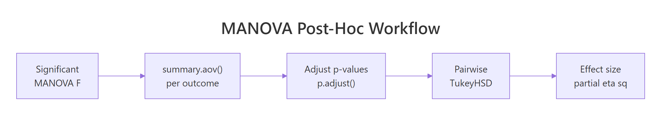
The full post-hoc workflow from a significant MANOVA to a journal-ready conclusion.

Figure 2: The full post-hoc workflow from a significant MANOVA to a journal-ready conclusion.

Step	R recipe
Per-outcome F-table	`summary.aov(manova_object)`
Extract raw p-values	`sapply(aov_summary, function(tab) tab[["Pr(>F)"]][1])`
Multiple-comparison correction	`p.adjust(p, method = "holm")` (or `"bonferroni"`, `"BH"`)
Pairwise contrasts (equal var.)	`TukeyHSD(aov(dv ~ group, data = ...))`
Pairwise contrasts (unequal var.)	`pairwise.t.test(..., pool.sd = FALSE, p.adjust.method = "holm")`
Variance-homogeneity check	`bartlett.test(dv ~ group, data = ...)`
Effect size per outcome	$\eta^2_p = SS_\text{effect} / (SS_\text{effect} + SS_\text{error})$
Multivariate post-hoc view	`MASS::lda(group ~ dv1 + dv2 + ...)`
When to use Bonferroni	Few outcomes, confirmatory study
When to use Holm	Default for k ≤ 6, strict Type I control with more power than Bonferroni
When to use BH	Many outcomes, exploratory study, control FDR

References

Smith, K. N., Lamb, K. N., & Henson, R. K. (2020). Making Meaning out of MANOVA: The Need for Multivariate Post Hoc Testing in Gifted Education Research. Gifted Child Quarterly, 64(2), 96-115. Link
Holm, S. (1979). A simple sequentially rejective multiple test procedure. Scandinavian Journal of Statistics, 6(2), 65-70.
Benjamini, Y., & Hochberg, Y. (1995). Controlling the false discovery rate: a practical and powerful approach to multiple testing. Journal of the Royal Statistical Society Series B, 57(1), 289-300.
R Core Team. *?summary.aov and ?TukeyHSD in base R.* Link
Tabachnick, B. G., & Fidell, L. S. (2019). Using Multivariate Statistics, 7th edition. Pearson. Chapter 7 on MANOVA.
Penn State STAT 505. Lesson 8.5: Comparing Mean Vectors. Link
Datanovia. One-Way MANOVA in R. Link
Venables, W. N., & Ripley, B. D. (2002). Modern Applied Statistics with S, 4th edition. Springer. Chapter 12 on MASS::lda and discriminant analysis.

Continue Learning

MANOVA in R, the parent tutorial that fits the multivariate model this article picks up from. Read it first if manova() syntax or Pillai versus Wilks feels unfamiliar.
Post-Hoc Tests After ANOVA, deeper coverage of TukeyHSD(), Bonferroni, and pairwise contrasts in the single-outcome setting that the per-DV step here reduces to.
One-Way ANOVA in R, the single-outcome companion that each summary.aov() row corresponds to.

MANOVA Post-Hoc Analysis: Univariate Follow-Up Tests in R

Why do you need a post-hoc step after a significant MANOVA?

How do you correct for multiple comparisons across the univariate ANOVAs?

How do you run pairwise group comparisons within each significant outcome?

How do you measure and report MANOVA effect sizes?

When should you use descriptive discriminant analysis instead?

Practice Exercises

Exercise 1: Full post-hoc on the airquality Month effect

Exercise 2: A reusable post-hoc helper function

Complete Example

Summary

References

Continue Learning

Related Tutorials