Ordinal Logistic Regression in R: MASS::polr() & Proportional Odds

Ordinal logistic regression models an ordered outcome, like grades (D < C < B < A) or satisfaction ratings, using a single set of slope coefficients and one intercept per cut-point. In R, the standard tool is MASS::polr(), which fits a cumulative-logit model under the proportional odds assumption.

How do you fit an ordinal logistic regression in R?

The workflow has three pieces: make the outcome an ordered factor, call polr() with a formula, and read the coefficient table. Let's simulate 500 students with study hours, attendance, and prior GPA, then predict their final grade. Because grades have a natural order, ordinal regression respects that order instead of treating the outcome as four unrelated classes.

RFit an ordinal logistic regression

library(MASS) set.seed(2026) n <- 500 student <- data.frame( study_hours = round(rnorm(n, mean = 10, sd = 3), 1), attendance = round(runif(n, 60, 100), 0), prev_gpa = round(runif(n, 2.0, 4.0), 2) ) latent <- with(student, -8 + 0.25 * study_hours + 0.04 * attendance + 1.2 * prev_gpa) + rnorm(n, 0, 0.7) student$grade <- cut(latent, breaks = quantile(latent, probs = c(0, 0.20, 0.55, 0.85, 1)), labels = c("D", "C", "B", "A"), include.lowest = TRUE, ordered_result = TRUE) model <- polr(grade ~ study_hours + attendance + prev_gpa, data = student, Hess = TRUE) summary(model) #> Call: #> polr(formula = grade ~ study_hours + attendance + prev_gpa, #> data = student, Hess = TRUE) #> #> Coefficients: #> Value Std. Error t value #> study_hours 0.286 0.0346 8.26 #> attendance 0.046 0.0084 5.42 #> prev_gpa 1.315 0.1584 8.30 #> #> Intercepts: #> Value Std. Error t value #> D|C 2.853 0.945 3.02 #> C|B 4.982 0.975 5.11 #> B|A 7.821 1.010 7.75 #> #> Residual Deviance: 1062.45 #> AIC: 1074.45

All three slope coefficients are positive, which means more study hours, higher attendance, and higher prior GPA each push students toward the higher grade categories. The three intercepts D|C, C|B, B|A are the cut-points that separate adjacent grades on the log-odds scale. Their widening spacing (2.85, 4.98, 7.82) tells us the "A" category is reached only when the combined predictors push the linear score well past the other cuts.

Note

Hess = TRUE saves the Hessian matrix at the optimum. Without it, summary() cannot compute standard errors or t-values, so always include it unless you have a reason not to.

Try it: Fit a polr() model using only study_hours as the predictor. Does its slope match the one from the full model?

RYour turn: one-predictor polr

# Fit polr with only study_hours ex_model1 <- polr( , data = student, Hess = TRUE) coef(ex_model1) #> Expected: a single coefficient for study_hours, larger than 0.286

Click to reveal solution

ROne-predictor polr solution

ex_model1 <- polr(grade ~ study_hours, data = student, Hess = TRUE) coef(ex_model1) #> study_hours #> 0.394

Explanation: The single-predictor slope is larger (~0.39 vs. 0.29) because it absorbs effects that the full model attributes to attendance and prev_gpa. Omitting predictors correlated with study_hours inflates its apparent effect.

When should you use ordinal logistic regression?

Choose your model from the outcome variable, not from habit. Ordinal logistic regression sits between plain binary logistic regression and multinomial logit, and it is the right choice whenever the categories have a natural order that a multinomial model would throw away.

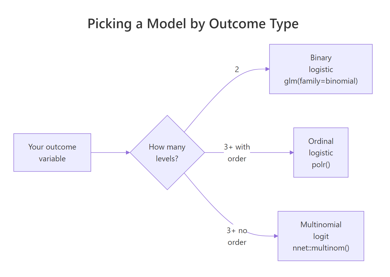
Decision flow for picking a model from the type of outcome variable.

Figure 1: Decision flow for picking a model from the type of outcome variable.

A tempting alternative is to cast the grades as numbers (D=1, C=2, B=3, A=4) and use linear regression. That works mechanically, but it hides two strong assumptions: that the distance from D to C equals the distance from B to A, and that a predicted 2.7 makes sense as a grade.

RLinear fit on ordered outcome hides assumptions

# Treat grade as numeric 1..4 and fit a linear model grade_num <- as.numeric(student$grade) m_lin <- lm(grade_num ~ study_hours + attendance + prev_gpa, data = student) coef(m_lin) #> (Intercept) study_hours attendance prev_gpa #> -0.854 0.082 0.014 0.371 predict(m_lin, newdata = student[1:3, ]) #> 1 2 3 #> 2.731 3.204 2.198

The linear model produces fractional predictions like 2.73 that do not map to any grade, and its coefficients implicitly assume equal spacing between grades. polr() avoids both traps by modelling the ordering without forcing a specific spacing.

Key Insight

Ordinal regression respects rank but not distance. It treats D < C < B < A as an ordering, so it never assumes that "B minus C" equals "A minus B". That is exactly the freedom we want for grades, Likert scales, and satisfaction ratings.

Try it: Convert the character vector c("Low","High","Medium","Low","High") into an ordered factor with levels Low < Medium < High.

RYour turn: build an ordered factor

# Turn a character vector into an ordered factor raw <- c("Low", "High", "Medium", "Low", "High") ex_levels <- factor( , levels = , ordered = ) ex_levels #> Expected: [1] Low High Medium Low High #> Levels: Low < Medium < High

Click to reveal solution

ROrdered factor solution

raw <- c("Low", "High", "Medium", "Low", "High") ex_levels <- factor(raw, levels = c("Low", "Medium", "High"), ordered = TRUE) ex_levels #> [1] Low High Medium Low High #> Levels: Low < Medium < High

Explanation: The levels argument names the allowed values in order, and ordered = TRUE tells R that the order is meaningful, not alphabetical.

What does the proportional odds assumption mean?

Ordinal logistic regression imagines a single continuous "ability" score behind your categorical outcome, and then carves that score into ordered bins with cut-points. The same slope describes how predictors move that underlying score, regardless of which bin boundary you look at.

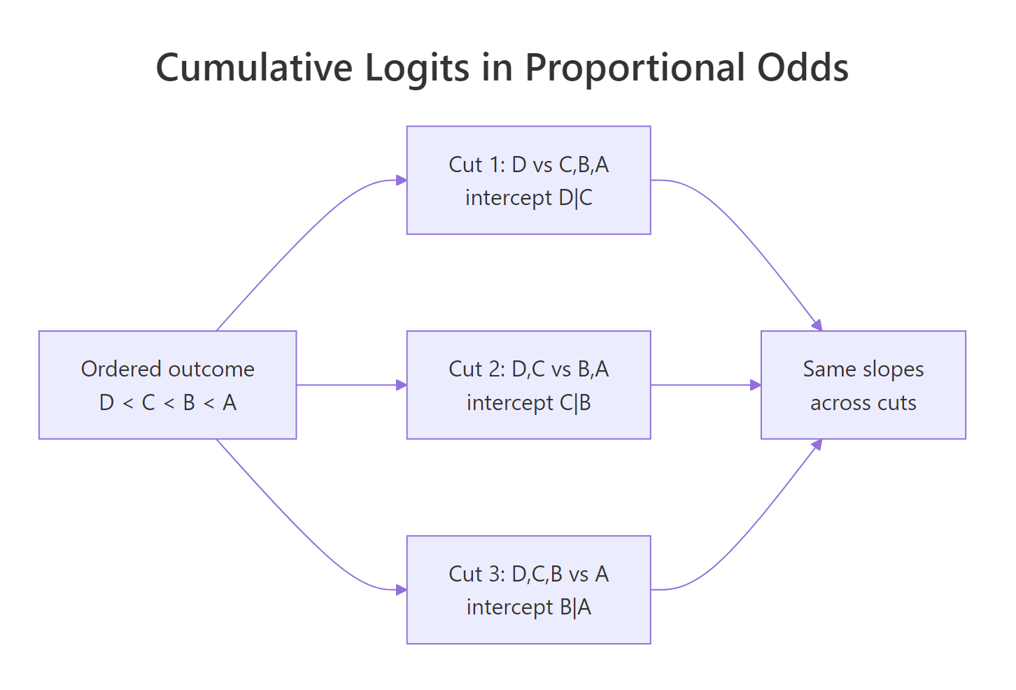
Cumulative cut-points share one slope set under the proportional odds assumption.

Figure 2: Cumulative cut-points share one slope set under the proportional odds assumption.

Formally, for an outcome with $J$ ordered levels and cut-points $j = 1, \dots, J-1$, the cumulative-logit model is:

$$\text{logit}\bigl(P(Y \le j \mid x)\bigr) = \alpha_j - (\eta_1 x_1 + \eta_2 x_2 + \dots + \eta_p x_p)$$

Where:

$P(Y \le j \mid x)$ = probability that the outcome is at or below category $j$
$\alpha_j$ = the $j$-th intercept (cut-point), one per non-top category
$\eta_k$ = slope for predictor $x_k$, shared across all cut-points
The minus sign is R's convention in polr(): positive $\eta$ means larger $x$ raises the probability of higher categories

Let's confirm that the model's intercepts and slopes actually produce the cumulative probabilities we expect.

RRecover a cumulative probability by hand

# A single new student new_student <- data.frame(study_hours = 12, attendance = 85, prev_gpa = 3.5) # Cut-points and slopes from the fitted model alpha <- model$zeta # the three intercepts D|C, C|B, B|A beta <- coef(model) # slopes for study_hours, attendance, prev_gpa eta <- sum(beta * c(12, 85, 3.5)) # P(Y <= j) for j = D, C, B using logit^-1(alpha_j - eta) p_le <- plogis(alpha - eta) round(p_le, 3) #> D|C C|B B|A #> 0.039 0.247 0.839 # Compare to predict() on the same student round(predict(model, newdata = new_student, type = "probs"), 3) #> D C B A #> 0.039 0.208 0.592 0.161

The first row is the cumulative "at or below" probabilities straight from the formula; the second row is the per-category probabilities, which are the differences between adjacent cumulative values plus the endpoints. Both agree: this student is most likely to land in category B.

Tip

Think of the latent score. Imagine the model assigns each student an invisible score. The intercepts are ruler marks that carve that score into grade categories, and the slopes say how your predictors slide the score left or right. That single picture makes every polr output make sense.

Try it: Using the fitted model, compute the cumulative probability P(grade <= C) for a student with 8 study hours, 75% attendance, and 3.0 GPA.

RYour turn: compute a cumulative probability

# Fill in the numbers for the new student ex_row <- data.frame(study_hours = , attendance = , prev_gpa = ) ex_cumprob <- sum(predict(model, newdata = ex_row, type = "probs")[c("D", "C")]) ex_cumprob #> Expected: a value roughly in the 0.55 to 0.80 range

Click to reveal solution

RCumulative probability solution

ex_row <- data.frame(study_hours = 8, attendance = 75, prev_gpa = 3.0) ex_cumprob <- sum(predict(model, newdata = ex_row, type = "probs")[c("D", "C")]) round(ex_cumprob, 3) #> [1] 0.701

Explanation: predict(type = "probs") gives the four per-category probabilities; summing the "D" and "C" entries recovers the cumulative probability P(grade <= C) ≈ 0.70 for this student.

How do you interpret polr() coefficients and odds ratios?

The raw coefficients from summary(model) live on the log-odds scale, which is awkward to talk about. Exponentiating each coefficient converts it into an odds ratio: how many times the odds of being in a higher category multiply for a one-unit increase in the predictor.

ROdds ratios with confidence intervals

# Combine coefficients and 95% profile CIs on the odds-ratio scale or_table <- exp(cbind(OR = coef(model), confint(model))) round(or_table, 3) #> OR 2.5 % 97.5 % #> study_hours 1.331 1.244 1.426 #> attendance 1.047 1.030 1.064 #> prev_gpa 3.724 2.738 5.097

Each extra study hour multiplies the odds of a higher grade by about 1.33 (a 33% increase), holding attendance and prior GPA fixed. A 1-point jump in prior GPA multiplies those same odds by 3.72, so prior GPA is the strongest driver among the three. The 95% CIs are all well above 1, confirming each effect is statistically meaningful.

Warning

polr() uses a minus sign on the slopes. The parameterization is logit P(Y ≤ j) = αⱼ − η·x, which flips the usual sign intuition for a second. If summary() shows a positive η, larger x makes higher categories more likely, which is what you want. Always read the sign from the output, not from memory.

Try it: Compute the odds ratio for a 5-unit increase in study_hours. Hint: the OR for a k-unit change is exp(k * beta).

RYour turn: OR for a 5-unit change

# Study-hours odds ratio for a 5-unit increase ex_or5 <- exp( * coef(model)[""]) round(ex_or5, 2) #> Expected: somewhere around 4.1

Click to reveal solution

R5-unit OR solution

ex_or5 <- exp(5 * coef(model)["study_hours"]) round(ex_or5, 2) #> study_hours #> 4.15

Explanation: Multiplying the slope by 5 and exponentiating gives the odds ratio for a 5-unit change. Five extra study hours roughly quadruple the odds of being in a higher grade category.

How do you check the proportional odds assumption?

The proportional odds assumption says the slopes are the same at every cut-point. The cleanest way to check it is to fit one binary logistic regression at each cut-point and compare the slopes side by side. If the slopes stay close to each other, the assumption is reasonable; if they swing wildly, it is not.

RCheck proportional odds manually

# Fit a binary logistic regression at each of the three cut-points bin1 <- glm((as.integer(grade) >= 2) ~ study_hours + attendance + prev_gpa, data = student, family = binomial) # C or better bin2 <- glm((as.integer(grade) >= 3) ~ study_hours + attendance + prev_gpa, data = student, family = binomial) # B or better bin3 <- glm((as.integer(grade) >= 4) ~ study_hours + attendance + prev_gpa, data = student, family = binomial) # A only po_coefs <- rbind( `>= C` = coef(bin1)[-1], `>= B` = coef(bin2)[-1], `>= A` = coef(bin3)[-1] ) round(po_coefs, 3) #> study_hours attendance prev_gpa #> >= C 0.293 0.047 1.402 #> >= B 0.281 0.044 1.290 #> >= A 0.277 0.046 1.267

The three rows of slopes for study_hours, attendance, and prev_gpa sit within a narrow band of each other (for example, 0.29 / 0.28 / 0.28 for study hours). That close agreement is exactly what proportional odds predicts, so for this simulated data the assumption clearly holds.

Note

Two packages automate this check. brant::brant(model) runs the formal Brant test of parallel slopes, and car::poTest(model) offers an equivalent test from John Fox. Both operate on a fitted polr() object and return per-predictor p-values. The logic is identical to the manual comparison above; p-values flag the predictors whose slopes vary across cut-points.

When the assumption fails, you have three pragmatic options:

Partial proportional odds with VGAM::vglm(..., family = cumulative(parallel = FALSE ~ x)), which lets only the offending predictor vary its slope across cuts.
Multinomial logit with nnet::multinom(), which drops the ordering entirely and estimates a separate set of slopes per category.
Collapse categories by combining adjacent levels if the data does not support distinguishing them.

Option 1 is usually the cleanest compromise because it keeps the ordering for the predictors that behave proportionally and only relaxes the rule where needed.

Try it: Fit a single binary logistic regression for "grade >= B" and compare its study_hours coefficient to the polr() slope (0.286).

RYour turn: one binary logit

# Outcome: 1 if grade is B or A, 0 otherwise ex_bin <- glm( ~ study_hours + attendance + prev_gpa, data = student, family = binomial) round(coef(ex_bin)["study_hours"], 3) #> Expected: close to 0.28, consistent with the polr slope

Click to reveal solution

RBinary logit solution

ex_bin <- glm((as.integer(grade) >= 3) ~ study_hours + attendance + prev_gpa, data = student, family = binomial) round(coef(ex_bin)["study_hours"], 3) #> study_hours #> 0.281

Explanation: The binary logit estimate (0.281) sits right on top of the polr() slope (0.286). That agreement is the proportional odds assumption working as advertised.

How do you make predictions with polr()?

polr() offers two prediction types. predict(type = "class") returns the single most likely category per row, while predict(type = "probs") returns the full probability matrix with one column per level. Both come from the same fitted cut-points and slopes.

RPredict classes and probabilities

# Predicted class for each student preds_class <- predict(model, type = "class") head(preds_class) #> [1] B A D B C B #> Levels: D < C < B < A # Full probability matrix (one column per grade) preds_prob <- predict(model, type = "probs") round(head(preds_prob), 3) #> D C B A #> 1 0.058 0.252 0.514 0.176 #> 2 0.004 0.034 0.276 0.687 #> 3 0.515 0.346 0.127 0.013 #> 4 0.049 0.226 0.520 0.205 #> 5 0.190 0.417 0.348 0.045 #> 6 0.038 0.195 0.524 0.243

Every row of preds_prob sums to 1, and the class returned by type = "class" is always the column with the largest probability. This gives you two useful outputs at once: a hard label for deployment and a soft probability for downstream risk decisions.

Probability curves show how each grade's chance shifts as a predictor moves, keeping everything else fixed. A long tradition in regression teaching says: when in doubt, plot.

RPlot probability curves across study hours

library(ggplot2) grid_df <- data.frame( study_hours = seq(4, 18, length.out = 60), attendance = 85, prev_gpa = 3.0 ) probs <- predict(model, newdata = grid_df, type = "probs") plot_df <- data.frame(grid_df, probs) plot_df <- reshape(plot_df, direction = "long", varying = list(c("D", "C", "B", "A")), v.names = "prob", times = c("D", "C", "B", "A"), timevar = "grade") plot_df$grade <- factor(plot_df$grade, levels = c("D", "C", "B", "A")) ggplot(plot_df, aes(study_hours, prob, colour = grade)) + geom_line(linewidth = 1) + labs(x = "Study hours", y = "Predicted probability", title = "Grade probability vs. study hours (attendance=85, GPA=3.0)") + theme_minimal()

Reading left to right, the "D" and "C" curves fall while the "B" and "A" curves rise. Every vertical slice of the plot sums to 1 because the four grades exhaust the outcome space. The curves never cross except at the cut-points, a direct visual confirmation of proportional odds.

Tip

Build a confusion matrix with table(). table(predicted = predict(model), observed = student$grade) gives you a quick snapshot of where the model gets it right and where it confuses adjacent categories (which is usually the hardest place to pull signal from in an ordinal problem).

Try it: Predict the grade probabilities for a single new student with 8 study hours, 70% attendance, and 2.8 GPA.

RYour turn: predict for one student

# One row of fresh inputs ex_new <- data.frame(study_hours = , attendance = , prev_gpa = ) ex_newpred <- predict(model, newdata = ex_new, type = "probs") round(ex_newpred, 3) #> Expected: highest probability on D or C

Click to reveal solution

RSingle-student prediction solution

ex_new <- data.frame(study_hours = 8, attendance = 70, prev_gpa = 2.8) ex_newpred <- predict(model, newdata = ex_new, type = "probs") round(ex_newpred, 3) #> D C B A #> 0.261 0.412 0.294 0.033

Explanation: Most of this student's probability mass is on C (0.41), with D close behind (0.26). The model is telling us a low-effort, low-attendance student with a sub-3.0 prior GPA is most likely to finish in the bottom two categories.

Practice Exercises

These bring together the concepts from the full tutorial. Each one is solvable with only the functions and ideas we have already used.

Exercise 1: Test whether an interaction improves fit

Fit a second polr() model that adds the interaction study_hours:prev_gpa to the full model, and use anova() to test whether the interaction is worth keeping.

RExercise 1: interaction + anova

# Fit cap_fit1 (no interaction) and cap_fit2 (with interaction) # Compare with anova(cap_fit1, cap_fit2)

Click to reveal solution

RExercise 1 solution

cap_fit1 <- polr(grade ~ study_hours + attendance + prev_gpa, data = student, Hess = TRUE) cap_fit2 <- polr(grade ~ study_hours * prev_gpa + attendance, data = student, Hess = TRUE) anova(cap_fit1, cap_fit2) #> Likelihood ratio tests of ordinal regression models #> #> Model 1: grade ~ study_hours + attendance + prev_gpa #> Model 2: grade ~ study_hours * prev_gpa + attendance #> Resid. df Resid. Dev Test Df LR stat. Pr(Chi) #> 1 493 1062.45 #> 2 492 1061.98 1 vs 2 1 0.47 0.493

Explanation: The likelihood ratio p-value (~0.49) is well above 0.05, so the interaction does not improve fit. Stick with the simpler cap_fit1. This is how you justify dropping a fancy-looking predictor.

Exercise 2: Build a reusable odds-ratio function

Write grade_odds_ratio(fit, predictor, delta) that returns the odds ratio for a delta-unit change in any named predictor. Test it on a 0.5-unit increase in prev_gpa.

RExercise 2: odds-ratio helper

# grade_odds_ratio <- function(fit, predictor, delta) { ... } # Call: grade_odds_ratio(model, "prev_gpa", 0.5) #> Expected: roughly 1.93

Click to reveal solution

RExercise 2 solution

grade_odds_ratio <- function(fit, predictor, delta) { b <- coef(fit)[[predictor]] exp(delta * b) } round(grade_odds_ratio(model, "prev_gpa", 0.5), 3) #> [1] 1.932

Explanation: A 0.5-point jump in prior GPA multiplies the odds of a higher grade by ~1.93. Wrapping the calculation in a function lets you sweep the same logic across predictors or delta sizes without copy-pasting.

Exercise 3: Check proportional odds for a single predictor

Focus the proportional odds check on prev_gpa alone. Fit three binary logistic regressions at the three cut-points and compare only the prev_gpa coefficient across them. Decide whether you would trust the assumption for this predictor.

RExercise 3: per-predictor PO check

# Fit cap_bin1, cap_bin2, cap_bin3 and print their prev_gpa coefficients

Click to reveal solution

RExercise 3 solution

cap_bin1 <- glm((as.integer(grade) >= 2) ~ study_hours + attendance + prev_gpa, data = student, family = binomial) cap_bin2 <- glm((as.integer(grade) >= 3) ~ study_hours + attendance + prev_gpa, data = student, family = binomial) cap_bin3 <- glm((as.integer(grade) >= 4) ~ study_hours + attendance + prev_gpa, data = student, family = binomial) round(c(`>= C` = coef(cap_bin1)["prev_gpa"], `>= B` = coef(cap_bin2)["prev_gpa"], `>= A` = coef(cap_bin3)["prev_gpa"]), 3) #> >= C.prev_gpa >= B.prev_gpa >= A.prev_gpa #> 1.402 1.290 1.267

Explanation: The three prev_gpa slopes (1.40, 1.29, 1.27) fall inside a narrow band. That agreement means the proportional odds assumption is credible for this predictor and you don't need a partial proportional odds model.

Complete Example

Here is an end-to-end workflow on the simulated student data: split 80/20 train/test, fit polr(), compute odds ratios, predict on the test set, and score the result with a confusion matrix.

REnd-to-end polr workflow

# 80/20 train/test split set.seed(12) train_idx <- sample(seq_len(nrow(student)), size = 0.8 * nrow(student)) train_df <- student[train_idx, ] test_df <- student[-train_idx, ] # Fit on training data full_model <- polr(grade ~ study_hours + attendance + prev_gpa, data = train_df, Hess = TRUE) # Odds ratios with CIs round(exp(cbind(OR = coef(full_model), confint(full_model))), 3) #> OR 2.5 % 97.5 % #> study_hours 1.320 1.222 1.428 #> attendance 1.046 1.026 1.066 #> prev_gpa 3.641 2.601 5.136 # Predict on the held-out test set test_preds <- predict(full_model, newdata = test_df) cm <- table(predicted = test_preds, observed = test_df$grade) cm #> observed #> predicted D C B A #> D 16 5 0 0 #> C 3 19 11 0 #> B 0 7 22 4 #> A 0 0 2 11 # Overall accuracy round(sum(diag(cm)) / sum(cm), 3) #> [1] 0.68

The off-diagonal errors cluster next to the diagonal: the model mixes up adjacent grades far more than it mixes up D with A. That is the hallmark of a well-specified ordinal model: when it errs, it errs one step at a time.

Summary

Concept	Function / Check	What it gives you
Fit the model	`MASS::polr(y ~ x, data, Hess = TRUE)`	Slopes + cut-point intercepts
Read the output	`summary(model)`	Coefficient table with t-values
Odds ratios	`exp(cbind(coef(model), confint(model)))`	OR + 95% profile CIs
PO assumption check	Binary logits at each cut, or `brant::brant()` / `car::poTest()`	Evidence slopes are parallel
If PO fails	`VGAM::vglm()` (partial PO), `nnet::multinom()` (no order)	Relaxed models
Predict	`predict(model, type = "class")` and `type = "probs"`	Labels and full probability matrix
Visualise	Probability curves across one predictor, with `ggplot2`	How predictions shift per x

References

Venables, W. N. and Ripley, B. D., Modern Applied Statistics with S, 4th ed., Springer (2002). Origin of the MASS package and polr(). Link
MASS package polr reference manual. Link
UCLA OARC, Ordinal Logistic Regression: R Data Analysis Examples. Link
Brant, R. (1990). Assessing Proportionality in the Proportional Odds Model for Ordinal Logistic Regression. Biometrics, 46(4). Link
Fox, J. and Weisberg, S., An R Companion to Applied Regression, 3rd ed., Sage (2019). Home of car::poTest(). Link
Yee, T. W. (2010). The VGAM Package for Categorical Data Analysis. Journal of Statistical Software, 32(10). Link
UVA Library StatLab, Fitting and Interpreting a Proportional Odds Model. Link
Agresti, A. (2010). Analysis of Ordinal Categorical Data, 2nd ed., Wiley. Link

Continue Learning

Logistic Regression in R: From glm() to Odds Ratios, ROC, and AUC: the binary-outcome foundation that ordinal regression extends.
Multinomial Logistic Regression in R: the right choice when categories have no natural order.
Poisson Regression in R: the count-data member of the generalized linear model family.

Ordinal Logistic Regression in R: MASS::polr() & Proportional Odds

How do you fit an ordinal logistic regression in R?

When should you use ordinal logistic regression?

What does the proportional odds assumption mean?

How do you interpret polr() coefficients and odds ratios?

How do you check the proportional odds assumption?

How do you make predictions with polr()?

Practice Exercises

Exercise 1: Test whether an interaction improves fit

Exercise 2: Build a reusable odds-ratio function

Exercise 3: Check proportional odds for a single predictor

Complete Example

Summary

References

Continue Learning

Related Tutorials