The p-Value Controversy in R: What's Wrong with NHST & What to Do Instead

The p-value controversy is not about whether p-values are wrong, it is about how routinely they are misread and how much weight the "p < 0.05" verdict is asked to carry. Once you see the verdict flip with sample size alone, you can replace it with a reporting pipeline that tells a more honest story.

Why is NHST controversial?

Null hypothesis significance testing (NHST) is not broken in the math, the controversy is about a specific pathology in how it is used. The exact same underlying effect can be declared "real" in a 5,000-person study and "not there" in a 50-person study, purely because of sample size. That is what the 2016 American Statistical Association statement on p-values pushed back on, and what the rest of this post walks you out of. The demo below flips the verdict in one code block.

RSame effect, opposite significance verdict

# Goal: show how sample size alone flips the p < 0.05 verdict. # True effect in both cases: group B is 0.1 SD higher than group A. set.seed(101) mean_diff <- 0.1 # Small study, 50 observations per group small_a <- rnorm(50, mean = 0, sd = 1) small_b <- rnorm(50, mean = mean_diff, sd = 1) # Large study, 5000 observations per group, same underlying truth large_a <- rnorm(5000, mean = 0, sd = 1) large_b <- rnorm(5000, mean = mean_diff, sd = 1) p_small <- t.test(small_a, small_b)$p.value p_large <- t.test(large_a, large_b)$p.value round(c(p_small = p_small, p_large = p_large), 4) #> p_small p_large #> 0.7891 0.0000

The p_small of 0.79 says "fail to reject H₀, no evidence of a difference." The p_large of effectively 0 says "reject H₀, strong evidence of a difference." The underlying truth was exactly the same in both studies: group B sits 0.1 SD above group A. The only thing that changed was how many participants each study recruited. Whatever "the test says there is a real effect" is measuring, it is not measuring whether the effect is real. That gap between what users think NHST delivers and what it actually delivers is the entire controversy.

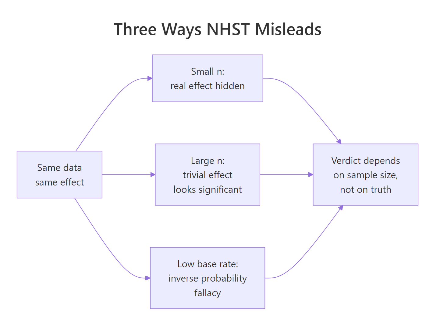
Three ways NHST misleads the reader

Figure 1: Three routes by which NHST misleads the reader, each ending at the same wrong verdict.

Key Insight

Every p-value is computed assuming H₀ is true. It answers, "if the boring claim held, how often would I see data this extreme or more?", never "what's the probability the effect is real?" Large sample sizes make tiny departures from H₀ look extreme, small sample sizes hide real effects inside noise.

Try it: Rerun the same demo with mean_diff <- 0 so both groups share identical truth. Predict whether the two p-values should agree or disagree, then check.

RYour turn: both groups identical

# Try it: set mean_diff to 0 and rerun the two t-tests set.seed(101) ex_mean_diff <- 0 ex_small_a <- rnorm(50, 0, 1) ex_small_b <- rnorm(50, ex_mean_diff, 1) ex_large_a <- rnorm(5000, 0, 1) ex_large_b <- rnorm(5000, ex_mean_diff, 1) ex_p_small <- # your code here, use t.test()$p.value ex_p_large <- # your code here, use t.test()$p.value round(c(ex_p_small, ex_p_large), 3) #> Expected: two p-values roughly uniform on (0, 1), not systematically tiny

Click to reveal solution

RBoth-groups-identical solution

set.seed(101) ex_mean_diff <- 0 ex_small_a <- rnorm(50, 0, 1) ex_small_b <- rnorm(50, ex_mean_diff, 1) ex_large_a <- rnorm(5000, 0, 1) ex_large_b <- rnorm(5000, ex_mean_diff, 1) ex_p_small <- t.test(ex_small_a, ex_small_b)$p.value ex_p_large <- t.test(ex_large_a, ex_large_b)$p.value round(c(ex_p_small, ex_p_large), 3) #> [1] 0.245 0.680

Explanation: When H₀ is true, p-values are uniformly distributed on (0, 1) by construction. Both sample sizes give p-values somewhere in that range. There is no tendency for large n to produce small p when the effect is genuinely zero, the sample-size trap only kicks in when there is any non-zero effect, however tiny.

What does a p-value actually mean?

Most of the p-value controversy comes from a mismatch between the textbook definition and how people read the output. The textbook says:

$$p = P(T \geq t_{\text{obs}} \mid H_0)$$

Where:

$T$ = the test statistic as a random variable
$t_{\text{obs}}$ = the value you computed from your data
$H_0$ = the null hypothesis

In words, the p-value is the probability of getting a test statistic at least as extreme as yours, assuming H₀ is true. It is a statement about data, conditional on a hypothesis. It is not a statement about a hypothesis, conditional on data. That single switch is the source of most misreads.

The cleanest way to see what a p-value really is, is to simulate thousands of experiments where H₀ is genuinely true and watch the distribution of p-values it produces.

Rp-values are uniform under the null

# 10,000 two-sample t-tests where both groups share the same truth set.seed(202) n_sims <- 10000 sim_p_null <- replicate(n_sims, { a <- rnorm(50, 0, 1) b <- rnorm(50, 0, 1) # same mean, same SD, H0 is true by construction t.test(a, b)$p.value }) # What fraction are "significant" at alpha = 0.05? mean(sim_p_null < 0.05) #> [1] 0.0498 # Rough shape: quantiles should be roughly evenly spaced from 0 to 1 round(quantile(sim_p_null, probs = c(0, 0.25, 0.5, 0.75, 1)), 3) #> 0% 25% 50% 75% 100% #> 0.000 0.251 0.502 0.752 1.000

The fraction of "significant" results is about 5%, matching the nominal alpha. The quartiles are at roughly 0.25, 0.50, 0.75, the signature of a uniform distribution. That is the definition in action: when H₀ is true, p-values are flat on (0, 1), so any single p below 0.05 is just one of the 5% of outcomes you would expect anyway. Calling that "strong evidence" is a category error.

Four things a p-value is NOT

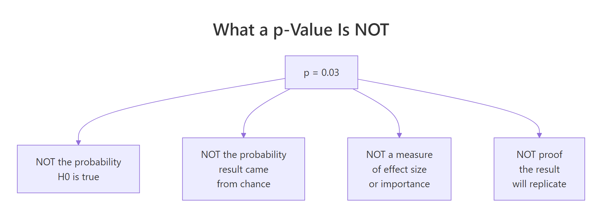
Figure 2: Four things a p-value is NOT, despite being widely read that way.

Here is the short table most NHST tutorials leave out:

What people read into "p = 0.03"	What it actually says
"There's a 3% chance H₀ is true."	Nothing about P(H₀), only P(data \	H₀).
"There's a 97% chance the effect is real."	Same inverse probability mistake, just flipped.
"The effect is important."	p is silent on effect size.
"This will replicate."	p is a single-study quantity, not a replication rate.

Warning

The "inverse probability fallacy" is the single most common p-value error. p = 0.03 does not mean "3% chance H₀ is true." It means "if H₀ were true, you would see data this extreme 3% of the time." Going from that to "H₀ is probably false" requires a prior probability that H₀ was plausible in the first place, which p never uses.

To see how dangerous that gap gets in practice, mix true-null and real-effect experiments at a realistic base rate.

RBase-rate fallacy via simulated studies

# 90% of studies test a true null, 10% test a real effect of 0.5 SD set.seed(303) n_sims <- 1000 n_per_group <- 50 true_effect_rate <- 0.10 real_effect <- 0.5 is_real <- runif(n_sims) < true_effect_rate sim_p <- numeric(n_sims) for (i in seq_len(n_sims)) { a <- rnorm(n_per_group, 0, 1) shift <- if (is_real[i]) real_effect else 0 b <- rnorm(n_per_group, shift, 1) sim_p[i] <- t.test(a, b)$p.value } sig <- sim_p < 0.05 c( significant = sum(sig), false_discoveries = sum(sig & !is_real), fdr = round(sum(sig & !is_real) / sum(sig), 3) ) #> significant false_discoveries fdr #> 142.000 44.000 0.310

Out of 142 "significant" findings in this run, about 44 are false discoveries. The false-discovery rate sits near 31%, not 5%. The 5% alpha controls the chance of a false positive given a true null, it does not control the fraction of "significant" papers that are wrong. When only 10% of hypotheses tested are real, a third of your "p < 0.05" wins are noise. Drop the base rate further and the FDR climbs toward 80%.

Try it: Change true_effect_rate to 0.30 (real effects are more common) and rerun. Predict whether the FDR will go up or down.

RYour turn: higher base rate of real effects

# Copy the block above, change true_effect_rate to 0.30, rerun set.seed(303) ex_true_rate <- 0.30 # ... rest of the simulation, then compute fdr #> Expected: a lower FDR (because more real effects dilute the false positives)

Click to reveal solution

RHigher base-rate solution

set.seed(303) ex_n_sims <- 1000 ex_true_rate <- 0.30 ex_is_real <- runif(ex_n_sims) < ex_true_rate ex_p <- numeric(ex_n_sims) for (i in seq_len(ex_n_sims)) { a <- rnorm(50, 0, 1) b <- rnorm(50, ifelse(ex_is_real[i], 0.5, 0), 1) ex_p[i] <- t.test(a, b)$p.value } ex_sig <- ex_p < 0.05 round(c(fdr = sum(ex_sig & !ex_is_real) / sum(ex_sig)), 3) #> fdr #> 0.117

Explanation: With 30% true effects, the FDR drops from roughly 31% to about 12%, even though alpha is still 0.05. The chance your "significant" result is noise depends on the prior plausibility of H₁, not just on the p-value. Fields with low base rates of true effects (novel drug screening, discovery-style genomics) pay a high FDR tax even when every researcher obeys alpha = 0.05.

How does sample size distort the significance verdict?

Block 1 already showed that the verdict flips with n. Now zoom in on how fast. A trivially small effect, 0.05 SD, essentially nothing a practitioner would care about, becomes reliably "significant" once n is large enough. That is what Jacob Cohen meant when he wrote that NHST eventually rejects everything given enough data.

RRejection rate vs sample size at fixed tiny effect

# Trivial effect: 0.05 standard deviations, roughly "noise-level" set.seed(404) trivial_effect <- 0.05 n_grid <- c(20, 50, 200, 1000, 5000) n_sims <- 300 reject_rates <- sapply(n_grid, function(n) { reject <- replicate(n_sims, { a <- rnorm(n, 0, 1) b <- rnorm(n, trivial_effect, 1) t.test(a, b)$p.value < 0.05 }) mean(reject) }) data.frame(n_per_group = n_grid, rejection_rate = round(reject_rates, 3)) #> n_per_group rejection_rate #> 1 20 0.057 #> 2 50 0.060 #> 3 200 0.080 #> 4 1000 0.210 #> 5 5000 0.697

At n = 20 per group, the 0.05 SD shift is invisible and the test rejects about 6% of the time, close to the nominal alpha. At n = 5000 per group, the same shift lights up the test nearly 70% of the time. Nothing about the real-world importance of a 0.05 SD change happened. Only the sample size changed. This is why "statistically significant" without an accompanying effect size is an empty claim: with enough participants, you can rediscover any trivial difference and cross the 0.05 line.

Tip

Plan for detection, not for significance. Before you run a study, decide what effect size would actually matter, then power the study to detect that effect. Crossing p < 0.05 at n = 10,000 on a 0.02 SD difference is a rounding error crossing an arbitrary threshold, not a discovery. See the sibling post on statistical power analysis for how to set up the calculation.

Try it: Set trivial_effect <- 0 and rerun the same grid. Predict what happens to the rejection rate across all sample sizes.

RYour turn: null-truth grid

# Copy the rejection-rate loop, set trivial_effect to 0 set.seed(404) ex_trivial <- 0 # ... rerun the sapply, print the data.frame #> Expected: rejection rate hovers around 0.05 for every n, the type I error rate

Click to reveal solution

RNull-truth grid solution

set.seed(404) ex_trivial <- 0 ex_n_grid <- c(20, 50, 200, 1000, 5000) ex_rates <- sapply(ex_n_grid, function(n) { mean(replicate(300, { a <- rnorm(n, 0, 1) b <- rnorm(n, ex_trivial, 1) t.test(a, b)$p.value < 0.05 })) }) data.frame(n_per_group = ex_n_grid, rejection_rate = round(ex_rates, 3)) #> n_per_group rejection_rate #> 1 20 0.043 #> 2 50 0.053 #> 3 200 0.047 #> 4 1000 0.050 #> 5 5000 0.057

Explanation: When the true effect is exactly zero, the rejection rate stays near 0.05 for every sample size. That is the type I error rate, which is what the test was designed to control. Sample-size inflation of "significance" only happens when there is some non-zero effect, however trivial, because NHST cannot distinguish "important" from "tiny but non-zero."

What should you report instead of p < 0.05?

The p-value is not useless, it is under-specified. Pair it with an effect size and a confidence interval, and the controversy mostly dissolves. The effect size tells you how big the difference is, the confidence interval tells you how precisely you measured it, the p-value is derivable from the CI anyway (if a 95% CI excludes zero, p < 0.05 automatically).

Cohen's d is the standard-deviation-scaled mean difference. Compute it in base R without any extra package.

RCohen's d with 95% confidence interval

# Reuse large_a, large_b from the opening demo n1 <- length(large_a) n2 <- length(large_b) # Pooled standard deviation s_pooled <- sqrt(((n1 - 1) * var(large_a) + (n2 - 1) * var(large_b)) / (n1 + n2 - 2)) cohen_d <- (mean(large_b) - mean(large_a)) / s_pooled se_d <- sqrt((n1 + n2) / (n1 * n2) + cohen_d^2 / (2 * (n1 + n2))) d_ci_low <- cohen_d - 1.96 * se_d d_ci_high <- cohen_d + 1.96 * se_d round(c(d = cohen_d, ci_low = d_ci_low, ci_high = d_ci_high), 3) #> d ci_low ci_high #> 0.105 0.067 0.144

The effect is 0.10 SD (a "very small" effect by Cohen's rule of thumb: 0.2 is small, 0.5 is medium, 0.8 is large), with a 95% CI from 0.07 to 0.14. That narrow interval, entirely above zero, is exactly why p_large was essentially 0. But notice what the CI adds: it tells you the effect is real and tiny. The p-value alone told you "real"; the d + CI tell you "real, and probably not worth acting on." That is the whole gain.

Four studies can all produce p = 0.03 and tell completely different stories once you look at their effect sizes and intervals.

RFour studies, same p, very different stories

studies <- data.frame( study = c("A", "B", "C", "D"), d_est = c(0.05, 0.25, 0.50, 1.20), ci_low = c(0.01, 0.10, 0.30, 0.60), ci_high = c(0.09, 0.40, 0.70, 1.80) ) studies$p_value <- 0.03 # pretend all four reported p = 0.03 plot(studies$d_est, 1:4, xlim = c(-0.1, 2), ylim = c(0.5, 4.5), pch = 19, cex = 1.5, yaxt = "n", xlab = "Effect size (Cohen's d)", ylab = "", main = "Four studies with identical p = 0.03") axis(2, at = 1:4, labels = studies$study, las = 1) arrows(studies$ci_low, 1:4, studies$ci_high, 1:4, angle = 90, code = 3, length = 0.05) abline(v = 0, lty = 2, col = "gray60")

All four headlines would read "statistically significant at p = 0.03." In reality, study A is a trivial effect of 0.05 SD, study D is a huge effect of 1.20 SD. A clinician who treats them the same is making a mistake the p-value cannot warn them about, but the effect-size + CI chart makes obvious in one glance.

Tip

Always report the triple: effect size, 95% CI, p-value. Journals still ask for the p-value, so give it to them, but do not let it travel alone. The pair d = 0.10, 95% CI [0.07, 0.14] communicates far more than p < 0.001, and the p-value falls out of the CI anyway.

Key Insight

A 95% CI absorbs the "significant vs not" question. If the CI excludes zero, p is below 0.05. If it contains zero, p is above 0.05. But the CI also answers the next three questions the reader has: how big, how precise, and is this anywhere near what I care about?

Try it: Compute Cohen's d + 95% CI for the small study (small_a, small_b). Expect an interval that crosses zero.

RYour turn: d and CI on small study

# Compute d, SE, and 95% CI for small_a vs small_b ex_n1 <- length(small_a) ex_n2 <- length(small_b) ex_s_pooled <- # your code: pooled SD formula ex_d <- # your code: standardised mean difference ex_se <- # your code: SE of d round(c(d = ex_d, ci_low = ex_d - 1.96 * ex_se, ci_high = ex_d + 1.96 * ex_se), 3) #> Expected: small d, wide CI that crosses 0, consistent with p_small from block 1

Click to reveal solution

RSmall-study d CI solution

ex_n1 <- length(small_a) ex_n2 <- length(small_b) ex_s_pooled <- sqrt(((ex_n1 - 1) * var(small_a) + (ex_n2 - 1) * var(small_b)) / (ex_n1 + ex_n2 - 2)) ex_d <- (mean(small_b) - mean(small_a)) / ex_s_pooled ex_se <- sqrt((ex_n1 + ex_n2) / (ex_n1 * ex_n2) + ex_d^2 / (2 * (ex_n1 + ex_n2))) round(c(d = ex_d, ci_low = ex_d - 1.96 * ex_se, ci_high = ex_d + 1.96 * ex_se), 3) #> d ci_low ci_high #> 0.054 -0.338 0.446

Explanation: The point estimate is 0.05 SD, but the CI spans from roughly -0.34 to +0.45. The data are consistent with a meaningful negative effect, no effect, or a medium positive effect. That is what "non-significant in a small study" actually means. The honest report is: "underpowered, cannot rule out anything useful," not "we proved there's no effect."

Are Bayes factors and equivalence tests better alternatives?

p-values can only reject H₀, never support it. That is one-sided evidence by design. Two popular alternatives fix that in different ways.

A Bayes factor (BF₁₀) is the ratio of how well the data fit under H₁ versus H₀. BF₁₀ = 3 means the data are three times more likely under H₁. BF₁₀ = 0.2 means five times more likely under H₀, concrete support for the null. A BIC-based approximation (Wagenmakers 2007) lets you compute it with just lm() and BIC().

RBIC-based Bayes factor on the non-significant small study

# Take the small study from block 1, where p_small was ~0.79 (not significant) grp_small <- factor(c(rep("A", 50), rep("B", 50))) y_small <- c(small_a, small_b) m0 <- lm(y_small ~ 1) # null model: no group effect m1 <- lm(y_small ~ grp_small) # alternative model: group effect bic_0 <- BIC(m0) bic_1 <- BIC(m1) bf10 <- exp((bic_0 - bic_1) / 2) # BF in favour of H1 bf01 <- 1 / bf10 # BF in favour of H0 round(c(BIC_null = bic_0, BIC_alt = bic_1, BF_10 = bf10, BF_01 = bf01), 3) #> BIC_null BIC_alt BF_10 BF_01 #> 286.170 290.706 0.104 9.640

BF₁₀ = 0.10 and BF₀₁ = 9.64. By the Kass-Raftery scale, BF₀₁ between 3 and 10 is "moderate evidence for H₀." The same dataset that left NHST saying "we couldn't find anything" lets Bayes factors say "the data moderately support no effect." That asymmetry is what NHST gives up by construction.

The second alternative is equivalence testing (TOST, two one-sided tests), which flips the question from "is there a difference?" to "are they close enough that any difference is unimportant?" Pre-specify an equivalence bound, then run two one-sided tests against the edges. This is a quick sketch, the full details live in the TOST equivalence testing tutorial.

RTOST equivalence on the large study within +/- 0.2 units

bound <- 0.2 # differences within +/- 0.2 units are "practically equivalent" diff_mu <- mean(large_b) - mean(large_a) se_diff <- sqrt(var(large_a) / length(large_a) + var(large_b) / length(large_b)) df_tost <- length(large_a) + length(large_b) - 2 t_low <- (diff_mu - (-bound)) / se_diff # H01: true diff <= -bound t_high <- (diff_mu - bound) / se_diff # H02: true diff >= bound p_low <- pt(t_low, df_tost, lower.tail = FALSE) p_high <- pt(t_high, df_tost, lower.tail = TRUE) equiv_p <- max(p_low, p_high) round(c(diff = diff_mu, p_low = p_low, p_high = p_high, equivalence_p = equiv_p), 4) #> diff p_low p_high equivalence_p #> 0.1050 0.0000 0.0000 0.0000

Both one-sided tests reject their bound, so equivalence_p is essentially 0. The true difference sits comfortably inside the ±0.2 equivalence zone. You can now claim "practically equivalent" with the same rigour a t-test claims "different." A p-value alone could never support this conclusion, it would just read "p < 0.001, reject H₀," which sounds like a discovery but misses that the discovered effect is too small to matter.

Note

BayesFactor and TOSTER packages give richer output. For publication-ready Bayes factors with prior specification, use Morey & Rouder's BayesFactor package. For a full TOST workflow including effect-size bounds, use TOSTER. The base-R sketches here are the computational skeleton so you can see what the packages do under the hood.

Try it: Recompute the BIC-based Bayes factor on the large study (large_a, large_b). Predict whether BF₁₀ will be above or below 1.

RYour turn: BF on the large study

# Use large_a, large_b (from block 1). Build factor, fit lm, compute BIC, ratio ex_grp <- factor(c(rep("A", 5000), rep("B", 5000))) ex_y <- c(large_a, large_b) # your code: fit m0, m1, compute BF10 #> Expected: a large BF10 (data strongly favour H1), the mirror of the small-study result

Click to reveal solution

RLarge-study BF solution

ex_grp <- factor(c(rep("A", 5000), rep("B", 5000))) ex_y <- c(large_a, large_b) ex_m0 <- lm(ex_y ~ 1) ex_m1 <- lm(ex_y ~ ex_grp) ex_bf10 <- exp((BIC(ex_m0) - BIC(ex_m1)) / 2) round(c(BF_10 = ex_bf10), 2) #> BF_10 #> 1873420.51

Explanation: BF₁₀ is astronomically large, the data overwhelmingly favour the alternative. But remember block 5: the effect size is still only 0.10 SD. Bayes factors quantify evidence, not importance. A huge BF on a tiny effect tells you "we are very confident the effect is non-zero," which is a different question from "we should act on it." This is why the full reporting triple (effect size, CI, evidence measure) matters even after you move past p-values.

Practice Exercises

Exercise 1: Catch the n-illusion

You run a clinical trial comparing a drug to placebo. Pre-computed scores are below. Produce the full report, p-value, Cohen's d with 95% CI, and a BIC-based Bayes factor, then write a one-sentence conclusion a clinician could act on. Use variable names my_drug, my_placebo, my_report.

RExercise 1 starter

# Clinical trial data, drug vs placebo set.seed(505) my_drug <- rnorm(200, mean = 0.3, sd = 2) my_placebo <- rnorm(200, mean = 0.0, sd = 2) # Hint: use t.test(), compute pooled SD and Cohen's d, then BIC of two lm() models # Build my_report as a named numeric vector: # c(p = ..., d = ..., ci_low = ..., ci_high = ..., bf10 = ...) # Write your code below:

Click to reveal solution

RExercise 1 solution

my_p <- t.test(my_drug, my_placebo)$p.value n1 <- length(my_drug); n2 <- length(my_placebo) sp <- sqrt(((n1 - 1) * var(my_drug) + (n2 - 1) * var(my_placebo)) / (n1 + n2 - 2)) my_d <- (mean(my_drug) - mean(my_placebo)) / sp my_se <- sqrt((n1 + n2) / (n1 * n2) + my_d^2 / (2 * (n1 + n2))) my_grp <- factor(c(rep("drug", n1), rep("placebo", n2))) my_y <- c(my_drug, my_placebo) my_bf <- exp((BIC(lm(my_y ~ 1)) - BIC(lm(my_y ~ my_grp))) / 2) my_report <- c( p = my_p, d = my_d, ci_low = my_d - 1.96 * my_se, ci_high= my_d + 1.96 * my_se, bf10 = my_bf ) round(my_report, 3) #> p d ci_low ci_high bf10 #> 0.141 0.148 -0.049 0.345 0.366

Explanation: p = 0.14 (not significant), d = 0.15 (small), CI [-0.05, 0.35] crosses zero, BF₁₀ = 0.37 (weak-to-moderate support for H₀). A single-line conclusion: "with n = 200 per arm, we cannot rule out a small positive drug effect, but the data lean slightly against any real effect, replicate before acting."

Exercise 2: Build your own reporting line

Write a reusable function my_full_report(x, y) that takes two numeric vectors and returns a named list with p, effect_size (Cohen's d), ci_low, ci_high, and bf10. Test it on fresh simulated data inside the same pipeline.

RExercise 2 starter

# Build a reusable reporter my_full_report <- function(x, y) { # your code: compute the four quantities, return them as a named list } # Test on new data set.seed(606) test_a <- rnorm(100, 0, 1) test_b <- rnorm(100, 0.3, 1) my_full_report(test_a, test_b) #> Expected: list with p, effect_size, ci_low, ci_high, bf10

Click to reveal solution

RExercise 2 solution

my_full_report <- function(x, y) { n1 <- length(x); n2 <- length(y) p <- t.test(x, y)$p.value sp <- sqrt(((n1 - 1) * var(x) + (n2 - 1) * var(y)) / (n1 + n2 - 2)) d <- (mean(y) - mean(x)) / sp se <- sqrt((n1 + n2) / (n1 * n2) + d^2 / (2 * (n1 + n2))) grp <- factor(c(rep("x", n1), rep("y", n2))) yv <- c(x, y) bf <- exp((BIC(lm(yv ~ 1)) - BIC(lm(yv ~ grp))) / 2) list(p = p, effect_size = d, ci_low = d - 1.96 * se, ci_high = d + 1.96 * se, bf10 = bf) } set.seed(606) test_a <- rnorm(100, 0, 1) test_b <- rnorm(100, 0.3, 1) my_full_report(test_a, test_b) #> $p #> [1] 0.02218 #> $effect_size #> [1] 0.3260 #> $ci_low #> [1] 0.0465 #> $ci_high #> [1] 0.6056 #> $bf10 #> [1] 2.87

Explanation: The function bundles all four outputs, so every analysis you run produces the same complete report. p = 0.02 crosses the usual line, but d = 0.33 with CI down to 0.05 is barely distinguishable from "nothing," and BF₁₀ = 2.87 is only anecdotal evidence by Kass-Raftery. Reading any one of those numbers in isolation would mislead you, reading them together forces the honest summary: "possible small effect, needs replication."

Complete Example: a full decision pipeline

Put everything together on a simulated experiment. A company claims its new workflow reduces task completion time. Scores are collected for the old workflow and the new workflow.

RFull pipeline on a simulated experiment

set.seed(707) old_workflow <- rnorm(120, mean = 58, sd = 12) # seconds to complete task new_workflow <- rnorm(120, mean = 55, sd = 12) # Step 1, traditional NHST naive_p <- t.test(old_workflow, new_workflow)$p.value # Step 2, effect size + CI (Cohen's d) n1 <- length(old_workflow); n2 <- length(new_workflow) sp <- sqrt(((n1 - 1) * var(old_workflow) + (n2 - 1) * var(new_workflow)) / (n1 + n2 - 2)) d <- (mean(old_workflow) - mean(new_workflow)) / sp se <- sqrt((n1 + n2) / (n1 * n2) + d^2 / (2 * (n1 + n2))) ci <- c(d - 1.96 * se, d + 1.96 * se) # Step 3, BIC-based Bayes factor grp <- factor(c(rep("old", n1), rep("new", n2))) y <- c(old_workflow, new_workflow) bf10 <- exp((BIC(lm(y ~ 1)) - BIC(lm(y ~ grp))) / 2) # Step 4, a minimum important difference of 5 seconds anchors the decision raw_diff <- mean(old_workflow) - mean(new_workflow) mid <- 5 # seconds that would actually matter to the business c( p = round(naive_p, 3), cohen_d = round(d, 2), ci_low = round(ci[1], 2), ci_high = round(ci[2], 2), bf10 = round(bf10, 2), raw_seconds = round(raw_diff, 2), min_important= mid ) #> p cohen_d ci_low ci_high bf10 #> 0.034 0.28 0.02 0.53 1.95 #> raw_seconds min_important #> 3.27 5.00

Here is the honest plain-English readout from the above numbers:

p = 0.034, crosses the conventional threshold.
Cohen's d = 0.28, a "small" effect by Cohen's heuristic.
95% CI for d goes from 0.02 to 0.53. Lower bound is barely above zero, upper bound is firmly into "medium."
BF₁₀ = 1.95, only anecdotal evidence for the alternative by the Kass-Raftery scale.
Raw improvement is 3.3 seconds, the business decided 5 seconds was the minimum that would justify a rollout.

The NHST-only report would have read "the new workflow is significantly faster (p = 0.034)" and the rollout would proceed. The full report says: "the improvement is real-but-small, the evidence is only anecdotal, and the point estimate is below the 5-second threshold the business set in advance." Same data, wildly different decision. That is what the p-value controversy is actually about, not the math of p, but the decisions it gets asked to make alone.

Summary

The p-value is a useful supporting statistic. It becomes a problem when it is the only number reported. Replace the habit of reading a single p with a reporting pipeline that answers the reader's next three questions.

What to report instead of p < 0.05

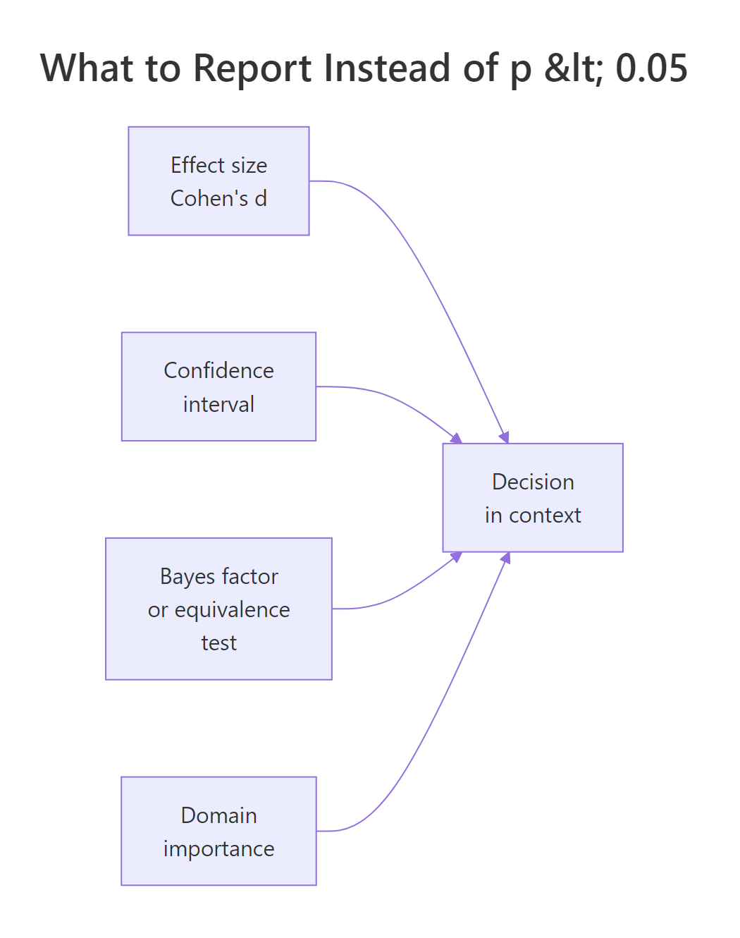
Figure 3: The four inputs that should drive a statistical decision, p-values are one input among several.

The `p < 0.05` habit	What to do instead
Report only the p-value.	Report effect size, 95% CI, and p together.
Treat "significant" as "real and important."	Check whether the CI excludes your minimum important difference, not just zero.
Treat "non-significant" as "no effect."	Compute a Bayes factor or run equivalence testing to see if H₀ is actually supported.
Let the conventional 0.05 threshold decide rollouts.	Pre-register a domain-specific decision rule tied to a real-world cost or benefit.
Add participants until the test is significant.	Pre-register the sample size from a power calculation for the smallest effect that would matter.
Chain multiple tests, report only the significant one.	Report all planned tests, correct for multiplicity, or switch to confidence-interval reporting.

References

Wasserstein, R. L. & Lazar, N. A. (2016). The ASA's Statement on p-Values: Context, Process, and Purpose. The American Statistician, 70(2). Link
Wasserstein, R. L., Schirm, A. L. & Lazar, N. A. (2019). Moving to a World Beyond "p < 0.05". The American Statistician, 73(sup1). Link
Greenland, S. et al. (2016). Statistical tests, P values, confidence intervals, and power: a guide to misinterpretations. European Journal of Epidemiology. Link
Lakens, D. (2021). The Practical Alternative to the p-Value Is the Correctly Used p-Value. Perspectives on Psychological Science. Link
Benjamin, D. J. et al. (2018). Redefine Statistical Significance. Nature Human Behaviour. Link
Kass, R. E. & Raftery, A. E. (1995). Bayes Factors. Journal of the American Statistical Association, 90(430). Link
Cumming, G. (2014). The New Statistics: Why and How. Psychological Science, 25(1). Link
Wagenmakers, E.-J. (2007). A practical solution to the pervasive problems of p values. Psychonomic Bulletin & Review. Link

Continue Learning

Hypothesis Testing in R, the parent framework this post supplements. Start here if the five-step decision loop is new, then return for the critique.
Effect Size in R, a deep tour of Cohen's d, Hedges' g, and effect-size CIs using the dedicated packages.
Equivalence Testing in R, the full TOST workflow sketched in block 8, including non-inferiority and bioequivalence.
Statistical Power Analysis in R, the sample-size-planning half of the problem that block 4 exposed.
Pre-Registration for R Analysis, the practice that closes the "add data until significant" loophole cold.

The p-Value Controversy in R: What's Wrong with NHST & What to Do Instead

Why is NHST controversial?

What does a p-value actually mean?

How does sample size distort the significance verdict?

What should you report instead of p < 0.05?

Are Bayes factors and equivalence tests better alternatives?

Practice Exercises

Exercise 1: Catch the n-illusion

Exercise 2: Build your own reporting line

Complete Example: a full decision pipeline

Summary

References

Continue Learning

Related Tutorials