Asymptotic Theory in R: Consistency, Asymptotic Normality & Delta Method

Asymptotic theory studies how estimators behave as the sample size grows. Three results do almost all the work in applied statistics: consistency (the estimator converges to the truth), asymptotic normality (it does so on a Gaussian scale after multiplying by $\sqrt{n}$), and the delta method (smooth transformations of asymptotically normal estimators are themselves asymptotically normal). This tutorial shows what each of them means by simulating all three in R.

What does it mean for an estimator to have good asymptotic behavior?

Large-sample guarantees let you trust a formula that would be hopeless to verify on one small sample. Instead of asking how good is my estimator at this sample size, asymptotic theory asks what happens as n grows without bound. We'll start with the most visible guarantee, consistency, and watch it in action by drawing samples of increasing size from a Normal distribution with known mean.

The absolute error shrinks by roughly a factor of 10 for every 100-fold increase in sample size, which is exactly the $1/\sqrt{n}$ rate we expect. At $n = 100{,}000$ the sample mean is off by less than 0.002 from the truth. That is consistency in one picture: the estimator homes in on the real parameter as more data arrives.

Formally, an estimator $\hat\theta_n$ is consistent for $\theta$ when it converges in probability:

$$\hat\theta_n \xrightarrow{\;p\;} \theta \quad \Longleftrightarrow \quad \lim_{n \to \infty} P(|\hat\theta_n - \theta| > \varepsilon) = 0 \text{ for every } \varepsilon > 0.$$

Where:

• $\hat\theta_n$ = the estimator computed from a sample of size $n$
• $\theta$ = the true parameter
• $\xrightarrow{p}$ = convergence in probability
• $\varepsilon$ = any small tolerance you pick

There are three properties asymptotic theory cares about:

1. Consistency, the estimator converges to the truth.
2. Asymptotic normality, rescaled errors $\sqrt{n}(\hat\theta_n - \theta)$ converge to a normal distribution.
3. Asymptotic efficiency, the asymptotic variance reaches the Cramér-Rao lower bound.

How do you verify consistency with a simulation in R?

A single shrinking error is convincing anecdotally, but consistency is a statement about the whole probability distribution of $\hat\theta_n - \theta$. The cleanest empirical check is to confirm that the mean squared error goes to zero. If MSE $\to 0$, then $\hat\theta_n \to_p \theta$ automatically (a standard result from Chebyshev's inequality). We'll estimate MSE at several sample sizes and plot it against $n$ on a log-log scale.

Empirical MSE tracks the theoretical value $\sigma^2/n$ almost exactly across two orders of magnitude in sample size. The ratio mse/theory stays within a few percent of 1, and both columns fall at the same rate. A log-log plot makes the rate visible at a glance.

The empirical and theoretical curves overlay perfectly, and the slope of the line is $-1$: doubling $n$ halves MSE. Any estimator whose MSE shrinks at this rate is consistent. If the slope were 0 (flat line), the estimator would be inconsistent.

What is asymptotic normality, and why does it matter?

Consistency tells you the estimator lands on the target eventually, but not how the errors are distributed. Asymptotic normality is the refinement that says: after you rescale $\hat\theta_n - \theta$ by $\sqrt{n}$, the distribution of the rescaled error approaches a Normal curve regardless of the population's shape. This is the statistical law that lets you build confidence intervals as $\hat\theta \pm 1.96 \times \text{SE}$ for almost every estimator you ever meet.

Formally, $\hat\theta_n$ is asymptotically normal with asymptotic variance $V$ when

$$\sqrt{n}\,(\hat\theta_n - \theta) \xrightarrow{\;d\;} N(0, V).$$

Where:

• $\xrightarrow{d}$ = convergence in distribution (the CDF of the left side converges to the CDF of the Normal)
• $V$ = the asymptotic variance (often called the "sandwich" variance for complicated models)
• The $\sqrt{n}$ factor is what makes the limit non-degenerate: without it, the left side would collapse to zero by consistency.

Let's see the central limit theorem deliver asymptotic normality for the sample mean. We'll draw 10,000 samples of size $n = 50$ from a skewed Gamma distribution, compute the standardized statistic $Z_n = \sqrt{n}(\bar{X}_n - \mu)/\sigma$, and overlay the histogram with the $N(0, 1)$ density.

The histogram is visually indistinguishable from the red Normal curve even though the raw Gamma data is skewed. Asymptotic normality doesn't care about the population distribution, only that it has finite variance. The $\sqrt{n}$ scaling is what produced the $N(0, 1)$ limit: without it, the numerator would shrink to zero.

A practical companion result is Slutsky's theorem: if you replace an unknown $V$ with a consistent estimator $\hat V$, the CI still has the right coverage. In other words, plug-in standard errors are asymptotically valid.

How does the delta method turn asymptotic normality into CIs for transformations?

You often need a CI not for $\theta$ itself but for some function $g(\theta)$: a log income, an odds ratio, a ratio of rates, a predicted probability. The delta method gives you the asymptotic distribution of $g(\hat\theta_n)$ for free, as long as $g$ is smooth at $\theta$. The idea is a one-term Taylor expansion: near $\theta$, $g(\hat\theta_n) \approx g(\theta) + g'(\theta)(\hat\theta_n - \theta)$. Combined with asymptotic normality of $\hat\theta_n$, this gives

$$\sqrt{n}\,(g(\hat\theta_n) - g(\theta)) \xrightarrow{\;d\;} N(0,\; [g'(\theta)]^2\, V).$$

Where:

• $g'(\theta)$ = the derivative of $g$ at the true parameter
• $V$ = the asymptotic variance of $\hat\theta_n$
• $[g'(\theta)]^2 V$ = the asymptotic variance of $g(\hat\theta_n)$

Let's check the formula with $g(\mu) = \log(\mu)$ on Normal data. The sample mean has asymptotic variance $V = \sigma^2$, and $g'(\mu) = 1/\mu$, so the delta method predicts an asymptotic variance of $\sigma^2 / \mu^2$ for $\log(\bar X_n)$. We simulate and compare.

Simulation and theory agree to about 1%. The delta method captures the spread of the log-transformed estimator almost perfectly. In practice this means you can write a Wald CI for $\log(\mu)$ as $\log(\bar X_n) \pm 1.96 \cdot (s / (\bar X_n \sqrt{n}))$, where $s$ is the sample SD plugged in for $\sigma$ (Slutsky again). Exponentiating the endpoints gives a back-transformed CI for $\mu$ that is valid asymptotically and often has better coverage than a naive CI built on the raw mean, especially for positive skewed data.

What does the multivariate delta method look like?

When the parameter is a vector $\boldsymbol\theta = (\theta_1, \dots, \theta_k)$ and $g$ is a real-valued function of the whole vector, the derivative $g'$ is replaced by the gradient $\nabla g$ and the variance $V$ becomes the asymptotic covariance matrix $\Sigma$. The multivariate delta method reads

$$\sqrt{n}\,(g(\hat{\boldsymbol\theta}_n) - g(\boldsymbol\theta)) \xrightarrow{\;d\;} N\!\big(0,\; \nabla g(\boldsymbol\theta)^\top\, \Sigma\, \nabla g(\boldsymbol\theta)\big).$$

Where:

• $\nabla g(\boldsymbol\theta)$ = the gradient vector of $g$ evaluated at the true parameter
• $\Sigma$ = the asymptotic covariance matrix of $\sqrt{n}(\hat{\boldsymbol\theta}_n - \boldsymbol\theta)$
• $\nabla g^\top \Sigma \nabla g$ = a scalar, the asymptotic variance of $g(\hat{\boldsymbol\theta}_n)$

A classic application is the log-odds-ratio from two independent Bernoulli samples. Let $\hat p_1$ and $\hat p_2$ be sample proportions from independent groups of size $n$ each, and define $g(p_1, p_2) = \log(p_1/(1-p_1)) - \log(p_2/(1-p_2))$. The gradient is $(1/[p_1(1-p_1)], -1/[p_2(1-p_2)])$. The asymptotic covariance is diagonal with entries $p_i(1-p_i)$, so the multivariate delta method collapses to a clean closed form.

The simulated variance (0.0293) sits on top of the delta-method prediction (0.0292), and the simulated mean matches the true log odds ratio. To build a 95% CI for the log-OR, you'd use $\hat\ell \pm 1.96 \sqrt{\hat V_{\text{dm}}}$ with $\hat p_i$ plugged into the formula (Slutsky again). Exponentiating gives a CI for the odds ratio itself.

Practice Exercises

Exercise 1: Fit the MSE decay slope

Compute the empirical MSE of the sample mean at $n = 20, 50, 100, 500, 1000$ from Normal(0, 3), then regress $\log_{10}(\text{MSE})$ on $\log_{10}(n)$. The fitted slope should be close to $-1$, confirming the $1/n$ rate and hence consistency.

Exercise 2: Delta-method CI for the coefficient of variation

The coefficient of variation is $\text{CV} = \sigma/\mu$. Its natural estimator is $\widehat{CV} = S / \bar X$. For Normal data the delta-method asymptotic variance works out to $\text{CV}^2 (1/(2) + \text{CV}^2)/n$ approximately, but we'll just estimate SE via simulation and build a Wald CI using the plug-in delta-method SE from a single sample. Evaluate coverage by drawing 2000 samples of size $n = 200$ from Normal(10, 2) and counting how often the delta-method 95% CI covers CV $= 0.2$.

Exercise 3: Detect delta-method failure at $g'(\theta) = 0$

Set $g(\mu) = \mu^2$ again, but this time with $\mu = 0$. Now $g'(\mu) = 2\mu = 0$, so the delta-method formula predicts zero asymptotic variance, which is clearly wrong. Simulate $\sqrt{n}\,\bar{X}_n^2$ at $n = 500$ from Normal(0, 1) and show the distribution is NOT normal; it is actually a scaled chi-square.

Complete Example: Delta-method CI for a ratio of means

Let's put every tool together. You have two independent samples of log-income (in log dollars), and you want a confidence interval for the ratio $\mu_1 / \mu_2$ of expected log-incomes. We'll use the multivariate delta method on the log scale to build a symmetric CI, then exponentiate, and compare against a bootstrap CI on the same data to sanity-check.

The delta-method CI and the bootstrap CI agree to the fourth decimal in both endpoints and width. That is the payoff of asymptotic theory: one derivative and one Normal quantile give you essentially the same interval a bootstrap would compute by resampling 2,000 times, at a tiny fraction of the cost. For large $n$ with smooth transformations, the delta method is virtually always the right first pass; you fall back to the bootstrap only when $n$ is small or the transformation is badly non-smooth.

Summary

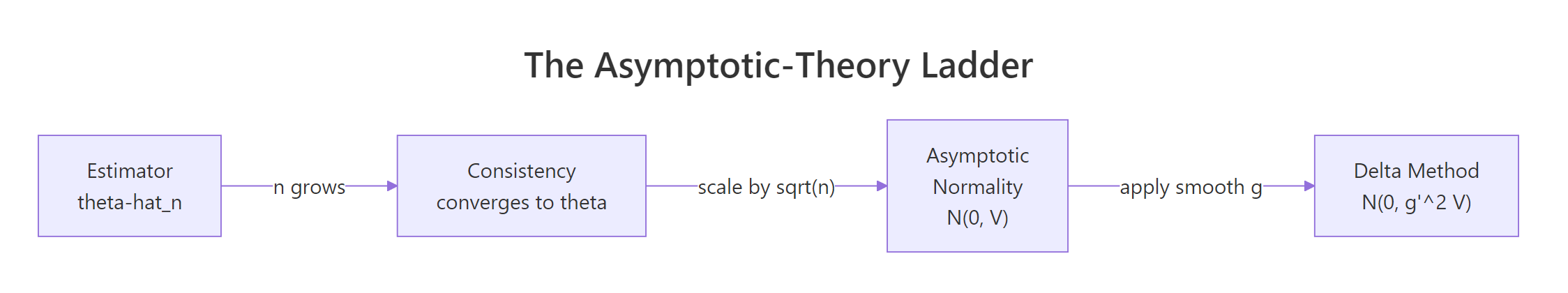
Figure 1: The asymptotic-theory ladder, climbed one rung at a time.

Think of it as a ladder. The first rung, consistency, guarantees you get to the right place. The second, asymptotic normality, guarantees the errors are shaped like a Gaussian on the $1/\sqrt{n}$ scale. The third, the delta method, extends the Gaussian story to any smooth function of the estimator. Together they explain why almost every inference in applied statistics takes the form $\hat\theta \pm 1.96 \times \text{SE}$.

References

1. van der Vaart, A. W., Asymptotic Statistics. Cambridge University Press (2000). Chapters 2 and 3. Link
2. Casella, G. & Berger, R. L., Statistical Inference, 2nd ed. Duxbury (2002). Chapter 10.
3. Lehmann, E. L., Elements of Large-Sample Theory. Springer (1999).
4. Wasserman, L., All of Statistics. Springer (2004). Chapter 5.
5. Wikipedia, "Delta method". Link
6. StatLect, "Delta method". Link
7. Stanford STATS 300A Lecture Notes, Large-sample theory.

Continue Learning

• Point Estimation in R: What Makes an Estimator Good?, the parent post covering bias, variance, and MSE for finite samples.
• Cramér-Rao Lower Bound in R, the variance floor that asymptotically efficient estimators reach.
• Central Limit Theorem in R, the flagship example of asymptotic normality in action.