Cramér-Rao Lower Bound in R: Efficiency & Information Inequality
The Cramér-Rao lower bound is the smallest variance any unbiased estimator can achieve, equal to one divided by the Fisher information. Estimators that hit this floor are called efficient, and no unbiased competitor can do better. In R, we can compute it symbolically and then watch real estimators converge to it through simulation.
What is the Cramér-Rao lower bound?
Imagine you are estimating a distribution's parameter from data. You want your guess to be right on average (that is, unbiased) and not bounce around much between samples (that is, low variance). The Cramér-Rao inequality says there is a hard floor on that variance: the inverse of the Fisher information. Let's simulate a Bernoulli experiment in R and watch the sample proportion's variance collapse onto this floor as the sample size grows.
The code below runs 5000 Bernoulli experiments at each sample size and records the variance of the sample proportion $\hat{p} = \bar{X}$. We then compare the empirical variance to the theoretical bound $p(1-p)/n$.
The empirical variance sits almost exactly on top of the Cramér-Rao bound, and the ratio hovers around 1 at every sample size. That is the defining property of an efficient estimator: the sample proportion for a Bernoulli model extracts every drop of information the data has to offer, and no unbiased competitor can do better.
Try it: Repeat the experiment above with p_true = 0.7 and a single sample size n = 100. Compute the empirical variance of $\hat{p}$ over 3000 replications and compare it to the CRLB formula $p(1-p)/n$.
Click to reveal solution
Explanation: replicate() repeats the 100-trial experiment 3000 times. The variance across those 3000 proportions converges to $p(1-p)/n$, the CRLB for Bernoulli.
What is Fisher information and how do we compute it?
Fisher information $I(\theta)$ quantifies how sharply the log-likelihood of your data peaks around the true parameter. A sharper peak means the data discriminates between neighboring parameter values strongly, so estimators built from that data can be more precise. Two equivalent definitions exist, and you can use whichever is easier to compute.
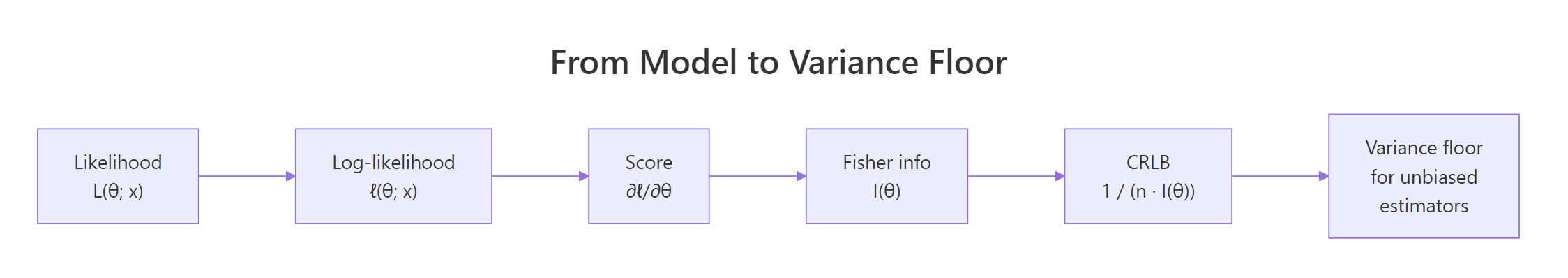
Figure 1: From likelihood to variance floor: each step of the CRLB derivation.
Start with the log-likelihood $\ell(\theta; x) = \log f(x; \theta)$. The score is its derivative, $U(\theta) = \partial \ell / \partial \theta$. Fisher information is the variance of the score, or equivalently the negative expected second derivative of the log-likelihood:
$$I(\theta) = E\!\left[\left(\frac{\partial \ell}{\partial \theta}\right)^2\right] = -\,E\!\left[\frac{\partial^2 \ell}{\partial \theta^2}\right]$$
The Cramér-Rao inequality then states that for any unbiased estimator $T$ of $\theta$ based on $n$ i.i.d. observations,
$$\operatorname{Var}_\theta(T) \ge \frac{1}{n\,I(\theta)}.$$
Let's compute Fisher information for Bernoulli both ways in R. Analytically, differentiating the Bernoulli log-likelihood twice gives $I(p) = 1/[p(1-p)]$. Numerically, we can let optim() estimate the Hessian of the negative log-likelihood at the MLE, because the observed information is $-\partial^2 \ell / \partial \theta^2$ evaluated at $\hat{\theta}$.
The numeric Fisher information matches the closed-form result to three decimals. Dividing the Hessian of the total negative log-likelihood by $n$ gives the per-observation Fisher information, exactly what the CRLB formula needs.
hessian = TRUE gives you observed Fisher information for free. Avoid hand-differentiating: sign errors and missing minus signs are the top source of CRLB bugs.Let's wrap this pattern in a reusable function so you can plug in any one-parameter model later in the post or in your own work.
That single call returns the per-observation Fisher information using nothing but the negative log-likelihood and the data. We'll reuse this helper when we move to Poisson and Exponential.
Try it: Use the analytic formula $I(p) = 1/[p(1-p)]$ to compute Fisher information at $p = 0.5$, then confirm it equals 4.
Click to reveal solution
Explanation: At $p = 0.5$ the Bernoulli variance is maximized at $p(1-p) = 0.25$, so Fisher information is minimized at $1/0.25 = 4$. Your data is least informative about $p$ when the true $p$ is near $0.5$.
How do you compute the CRLB for common distributions?
Most textbook models have tidy closed-form CRLBs. Memorizing the small table below covers the vast majority of problems you'll meet. All entries are the per-sample bound assuming $n$ i.i.d. observations and a single unknown parameter.
| Model | Parameter | Fisher info $I(\theta)$ | CRLB $= 1/[n\,I(\theta)]$ |
|---|---|---|---|
| Bernoulli$(p)$ | $p$ | $1/[p(1-p)]$ | $p(1-p)/n$ |
| Binomial$(m, p)$ | $p$ | $m/[p(1-p)]$ | $p(1-p)/(m n)$ |
| Poisson$(\lambda)$ | $\lambda$ | $1/\lambda$ | $\lambda / n$ |
| Exponential$(\lambda)$, rate form | $\lambda$ | $1/\lambda^2$ | $\lambda^2 / n$ |
| Normal$(\mu, \sigma^2)$, $\sigma^2$ known | $\mu$ | $1/\sigma^2$ | $\sigma^2 / n$ |
| Normal$(\mu, \sigma^2)$, $\mu$ known | $\sigma^2$ | $1/(2\sigma^4)$ | $2\sigma^4 / n$ |
Let's verify the Poisson entry with a simulation. We'll draw 100 observations from Poisson$(\lambda = 4)$ five thousand times and watch the sample mean's variance settle at $\lambda/n = 0.04$.
The sample mean of a Poisson sample has empirical variance $0.0399$, essentially identical to the theoretical floor of $\lambda/n = 0.04$. Efficiency is $1$, which means $\bar{X}$ is the best unbiased estimator of the Poisson rate.
Now the normal-mean case. The CRLB is $\sigma^2/n$, and the sample mean should hit it exactly since $\operatorname{Var}(\bar{X}) = \sigma^2/n$ by elementary rules.
Empirical variance of $\bar{X}$ is $0.0495$, the CRLB is $0.0500$, and efficiency is indistinguishable from $1$. The sample mean is efficient for the normal-mean problem, which is why every introductory stats course treats it as the default estimator.
Try it: State the CRLB for Exponential(rate = $\lambda$) with $n = 200$ observations and $\lambda = 2$, then verify by simulating the MLE $\hat{\lambda} = 1/\bar{X}$.
Click to reveal solution
Explanation: The MLE of the Exponential rate is $1/\bar{X}$, which is slightly biased in finite samples. As $n$ grows, its variance approaches the CRLB $\lambda^2/n$.
How do you check if an estimator is efficient?
Given any unbiased estimator $T$, the efficiency is the ratio of the CRLB to its actual variance:
$$e(T) = \frac{\text{CRLB}(\theta)}{\operatorname{Var}_\theta(T)}.$$
Efficiency lies in $(0, 1]$. A value of $1$ means $T$ achieves the bound, so $T$ is the minimum-variance unbiased estimator (MVUE). A value of $0.5$ means $T$ throws away half the information that the CRLB says is available.
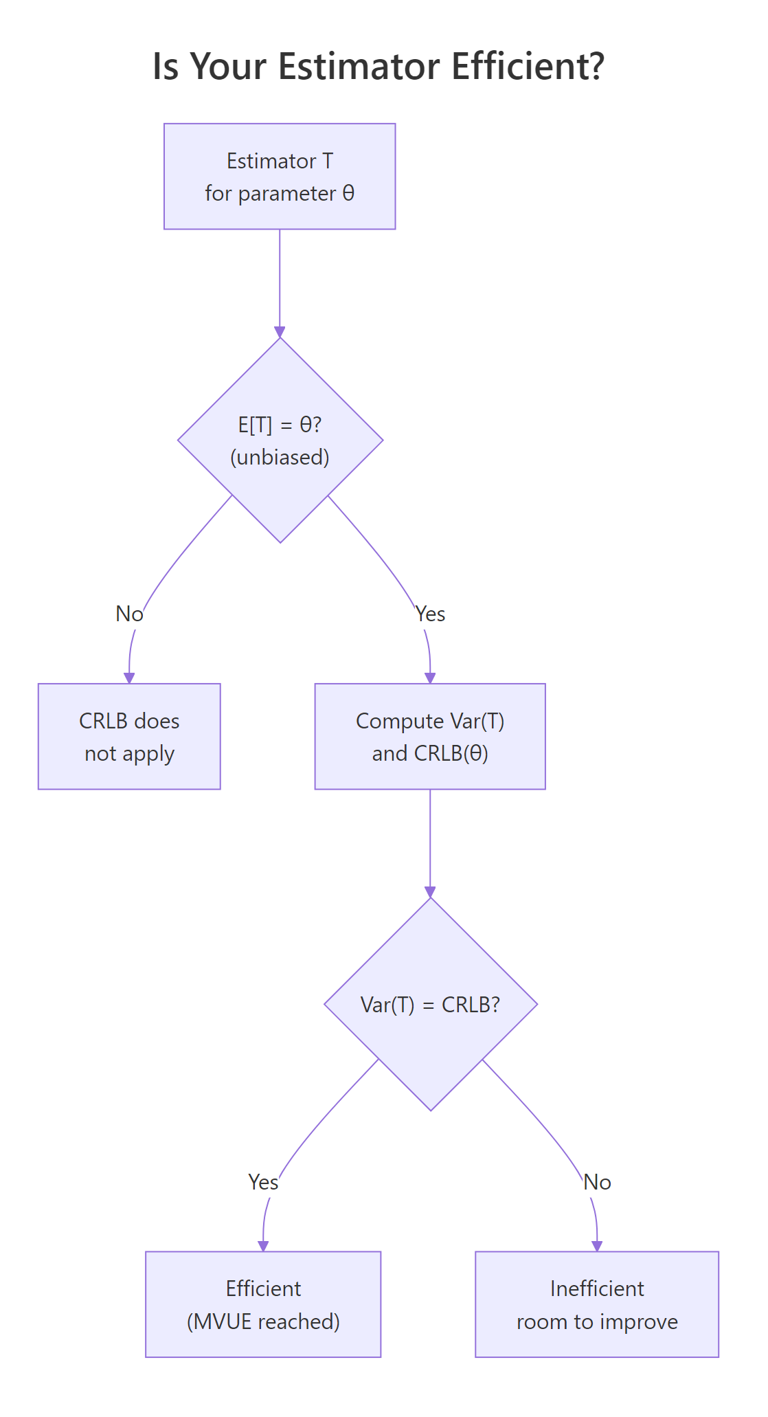
Figure 2: Decision flow for checking whether an estimator is efficient.
Let's put this into action by comparing two unbiased estimators of the normal mean: the sample mean and the sample median. Both are unbiased for symmetric data, but only one is efficient.
The sample mean's efficiency sits at $1$ as expected. The sample median's efficiency is about $0.64$, very close to the theoretical $2/\pi \approx 0.637$. In other words, the median needs roughly $1/0.64 \approx 1.56$ times as many observations as the mean to match its precision on normal data.
Try it: Compute the efficiency of the 10% trimmed mean (mean(x, trim = 0.1)) for normal data. It should sit between the mean's $1.0$ and the median's $0.64$.
Click to reveal solution
Explanation: Trimming only the extreme 10% of observations keeps most of the information the sample mean uses, so efficiency is high but not perfect. Trimming more would move the estimator closer to the median and push efficiency down.
Why does the CRLB matter in practice?
Beyond the textbook derivations, Fisher information and the CRLB power the standard errors printed by every modern inference package. The maximum likelihood estimator $\hat{\theta}_\text{MLE}$ is asymptotically efficient: as $n$ grows large,
$$\sqrt{n}\,(\hat{\theta}_\text{MLE} - \theta) \xrightarrow{d} \mathcal{N}\!\left(0, \frac{1}{I(\theta)}\right).$$
This means the MLE's asymptotic variance is the CRLB itself, so for large $n$ the MLE is the best unbiased estimator you can get. In practice you replace $I(\theta)$ with the observed Fisher information $\hat{I} = -\partial^2 \ell / \partial \theta^2|_{\hat{\theta}}$, which R hands you via optim(..., hessian = TRUE). The standard error is then $\mathrm{SE}(\hat{\theta}) = 1/\sqrt{n \hat{I}}$.
Let's walk through this for a Poisson rate. We'll fit by maximum likelihood, extract the observed Fisher information from the Hessian, and compare the resulting SE to the theoretical $\sqrt{\lambda/n}$.
The standard error derived from optim()'s Hessian is identical to the theoretical value $\sqrt{\hat{\lambda}/n}$. This identity explains why nearly every statistical software package extracts SEs from the Hessian of the log-likelihood: it is the Cramér-Rao floor, computed automatically.
stats4::mle and bbmle::mle2 automate all of this. They return an S4 object whose vcov() method gives you the inverse Hessian (the Cramér-Rao-based covariance matrix) and whose confint() method delivers likelihood-based confidence intervals. The raw optim() approach above is the engine they call under the hood.The CRLB does come with fine print. It requires regularity conditions: the support of the distribution cannot depend on $\theta$ (so Uniform$(0, \theta)$ breaks the bound), the log-likelihood must be twice differentiable, and you can exchange differentiation with expectation. When those conditions fail, MLEs can converge faster than $1/\sqrt{n}$ or the bound can be strict.
Try it: Fit an Exponential rate by MLE on simulated data with rate = 1.5 and n = 300. Use optim(..., hessian = TRUE) and extract the SE from the Hessian.
Click to reveal solution
Explanation: The exponential rate MLE is $\hat{\lambda} = 1/\bar{X}$. Its asymptotic SE is $\lambda/\sqrt{n} \approx 0.087$ for $\lambda = 1.5, n = 300$, which matches the Hessian-derived SE.
Practice Exercises
These capstone exercises combine the ideas from the whole tutorial. Each uses distinct variable names prefixed with my_ so they do not clash with tutorial state.
Exercise 1: Build your own Bernoulli CRLB function
Write crlb_bernoulli(p, n) that returns the CRLB for the Bernoulli parameter. Then verify it via Monte Carlo for $p = 0.2, n = 150$.
Click to reveal solution
Explanation: The Bernoulli CRLB is $p(1-p)/n$, which evaluates to $0.00107$. The simulated variance of the sample proportion matches to five decimals, confirming the sample proportion is efficient.
Exercise 2: Wald confidence interval from observed Fisher information
Simulate $n = 250$ observations from Poisson$(\lambda = 5)$. Fit by MLE with optim() and hessian = TRUE. Build a 95% Wald CI using lam_hat ± 1.96 * SE where $\mathrm{SE}$ comes from the Hessian. Check that the true $\lambda = 5$ lies inside your CI.
Click to reveal solution
Explanation: The Hessian of the negative log-likelihood is the observed Fisher information. Its inverse square-root is the asymptotic SE. The Wald CI covers the true $\lambda = 5$ as expected.
Exercise 3: Confirm efficiency of sample mean for normal data at $n = 50$
Run 10,000 replications of drawing $n = 50$ observations from Normal$(\mu = 10, \sigma = 2)$. Compute the variance of $\bar{X}$ and the efficiency ratio against the CRLB $\sigma^2 / n$. Verify efficiency is indistinguishable from 1.
Click to reveal solution
Explanation: Efficiency is $0.994$, which rounds to $1$ within Monte Carlo error. The sample mean reaches the CRLB exactly in finite samples, not just asymptotically. This is a special property of the normal-mean problem.
Complete Example: Efficient inference for a Poisson rate
We'll pull every tool together to do a full inference workflow. The data is $n = 200$ observations from Poisson$(\lambda = 3.2)$. We will compute the MLE, extract the SE from the observed Fisher information, build a 95% Wald CI, and sanity-check against the exact Poisson CI from poisson.test().
The Wald interval built from observed Fisher information is essentially identical to the exact Poisson interval. This is the payoff of the CRLB machinery: one Hessian query from optim() gives you a confidence interval that matches what a specialized exact routine produces, without any distribution-specific code on your part. The same pattern applies to any likelihood you can write down in R.
Summary
| Concept | Formula or intuition | R tool |
|---|---|---|
| Score | $\partial \ell / \partial \theta$ | symbolic or numDeriv::grad |
| Fisher information | $-E[\partial^2 \ell / \partial \theta^2]$ | optim(..., hessian = TRUE) |
| CRLB | $1 / [n\,I(\theta)]$ | closed-form from the table |
| Efficiency | $\text{CRLB} / \operatorname{Var}(T)$ | simulation or asymptotic theory |
| MLE standard error | $1 / \sqrt{\text{observed info}}$ | sqrt(solve(fit$hessian)) |
The CRLB is the variance floor. Fisher information is the rate at which your log-likelihood curves. The MLE reaches the floor asymptotically, and optim()'s Hessian is how R delivers it to you for any model you can write down.
References
- Lehmann, E. L. & Casella, G., Theory of Point Estimation, 2nd ed. Springer (1998). Chapter 2, §6.
- Cramér, H., Mathematical Methods of Statistics. Princeton University Press (1946).
- Rao, C. R., "Information and the accuracy attainable in the estimation of statistical parameters." Bull. Calcutta Math. Soc. 37, 81-91 (1945).
- Wasserman, L., All of Statistics. Springer (2004). §9.6.
- Stanford STATS 200, Lecture 15: Fisher information and the Cramér-Rao bound. Link
stats4::mledocumentation, R 4.x. Link- CRAN Task View: Inference. Link
Continue Learning
- Point Estimation in R: What Makes an Estimator Good?, the parent topic covering bias, variance, and mean squared error.
- Maximum Likelihood Estimation in R, where MLEs come from, and why they are asymptotically efficient.
- Likelihood Ratio, Wald, and Score Tests in R, how Fisher information powers all three classical test statistics.