Jackknife Resampling in R: Leave-One-Out Bias Correction

Jackknife resampling estimates the bias and standard error of a statistic by recomputing it on n leave-one-out subsamples: drop one observation, recompute, repeat. In base R, the whole machine is a five-line loop, and it returns the same standard error you would get from textbook formulas.

What is jackknife resampling, and how does it work?

The recipe is mechanical. Take a sample of n observations. Drop the first one and compute your statistic on the remaining n-1. Put it back, drop the second, repeat. After n passes you have n leave-one-out estimates, and their spread tells you how stable the original estimate is. Let's see this on the mean of mtcars$mpg, where the analytic standard error is already known.

RManual leave-one-out for the mean

x <- mtcars$mpg n <- length(x) theta_hat <- mean(x) # leave-one-out estimates jack_means <- sapply(1:n, function(i) mean(x[-i])) # jackknife standard error jack_se <- sqrt((n - 1) / n * sum((jack_means - mean(jack_means))^2)) # compare with the analytic standard error of the mean analytic_se <- sd(x) / sqrt(n) c(theta_hat = theta_hat, jack_se = jack_se, analytic_se = analytic_se) #> theta_hat jack_se analytic_se #> 20.09062 1.06542 1.06542

The two standard errors agree to every decimal. That is not a coincidence: for the sample mean, the jackknife formula reduces algebraically to sd(x)/sqrt(n). This match is the sanity check that anchors the rest of the method, and it works without us having to write down a single distributional assumption.

Jackknife leave-one-out flow.

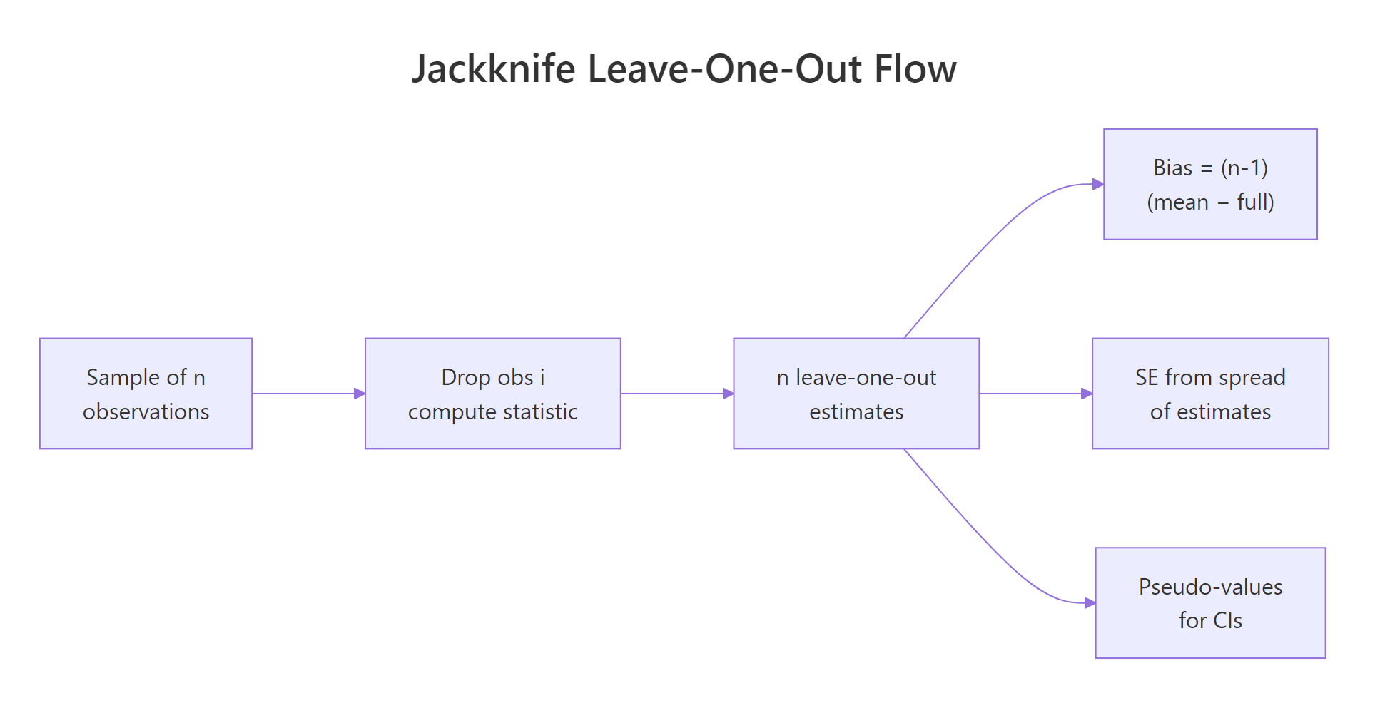
Figure 1: How n leave-one-out samples produce n estimates and one summary.

The math behind jack_se is a single formula:

$$\text{SE}_\text{jack} = \sqrt{\frac{n-1}{n} \sum_{i=1}^{n} \left( \hat\theta_{(-i)} - \bar{\theta}_\text{jack} \right)^2}$$

Where:

$\hat\theta_{(-i)}$ = the estimate computed on the sample with observation $i$ removed
$\bar{\theta}_\text{jack}$ = the average of those n leave-one-out estimates
The (n-1)/n factor inflates the spread to compensate for the high correlation between leave-one-out subsamples (they overlap in n-2 observations).

Let's wrap that loop in a tiny reusable function, since we'll need it again for bias and confidence intervals.

RReusable jack() helper

jack <- function(v, statistic) { nn <- length(v) values <- sapply(1:nn, function(i) statistic(v[-i])) list( value = statistic(v), values = values, mean = mean(values), se = sqrt((nn - 1) / nn * sum((values - mean(values))^2)) ) } jack(mtcars$mpg, mean)$se #> [1] 1.06542

The helper returns the original estimate, all n leave-one-out values, their mean, and the jackknife standard error. We'll reuse it across every section without rebuilding the loop.

Key Insight

The jackknife standard error of the sample mean equals the analytic standard error. This is an algebraic identity, not an empirical curiosity, and it is the reason the jackknife is treated as a credible substitute when no closed-form standard error exists.

Try it: Use jack() to estimate the standard error of the median of mtcars$wt. Print the SE.

RYour turn: jackknife SE for the median

# Try it: jackknife the median of mtcars$wt ex_w <- mtcars$wt # your code here #> Expected: a single numeric SE

Click to reveal solution

RMedian SE solution

ex_jack_med <- jack(ex_w, median) ex_jack_med$se #> [1] 0.2868649

Explanation: jack() plugs median into the same loop. Hold on to this number, we'll see in the last section that the jackknife standard error for the median is unreliable for a different reason.

How do you estimate bias with the jackknife?

A statistic is biased if its expected value over repeated sampling differs from the true population value. The jackknife estimates that bias from a single sample using a striking formula:

$$\text{bias}_\text{jack} = (n-1) \left( \bar{\theta}_\text{jack} - \hat\theta \right)$$

Where:

$\hat\theta$ = the estimate on the full sample
$\bar{\theta}_\text{jack}$ = the average of the n leave-one-out estimates

The bias-corrected estimator is then:

$$\hat\theta^{*}_\text{jack} = n\hat\theta - (n-1)\bar{\theta}_\text{jack}$$

A clean place to test this is the textbook biased variance: dividing by n instead of n-1 is known to underestimate the population variance by exactly $\sigma^2/n$. The jackknife should detect that bias and undo it.

RBias-correct a biased variance estimator

biased_var <- function(v) sum((v - mean(v))^2) / length(v) bv_naive <- biased_var(x) bv_jack <- jack(x, biased_var) bias_estimate <- (n - 1) * (bv_jack$mean - bv_naive) bv_corrected <- n * bv_naive - (n - 1) * bv_jack$mean c(bv_naive = bv_naive, bias_estimate = bias_estimate, bv_corrected = bv_corrected, unbiased_var = var(x)) #> bv_naive bias_estimate bv_corrected unbiased_var #> 35.18897 -1.13513 36.32411 36.32411

The corrected estimate matches var(x) exactly. The jackknife discovered the 1/n versus 1/(n-1) mistake on its own, with no knowledge of the analytic correction. The bias estimate is negative because the naive estimator underestimates the true variance.

The same technique works for statistics whose bias has no clean closed form, like Pearson's correlation, which is mildly biased toward zero in small samples.

RBias of Pearson correlation

mpg <- mtcars$mpg wt <- mtcars$wt r_naive <- cor(mpg, wt) # leave-one-out correlations jack_r <- sapply(1:n, function(i) cor(mpg[-i], wt[-i])) r_bias_estimate <- (n - 1) * (mean(jack_r) - r_naive) r_corrected <- n * r_naive - (n - 1) * mean(jack_r) c(r_naive = r_naive, r_bias = r_bias_estimate, r_corrected = r_corrected) #> r_naive r_bias r_corrected #> -0.86765938 -0.00355891 -0.87121829

The bias is small, around three thousandths, but it consistently pushes the estimate toward zero. The corrected value is very slightly more negative, in line with the well-known small-sample bias of cor(). With n = 32 you would not lose sleep over the gap, but with n = 10 the same correction can move an estimate by 0.05 or more.

Tip

Bias correction is not always a free lunch. The corrected estimator can have higher variance than the naive one, so you can trade a small bias reduction for a larger MSE. Apply the correction when n is small or when bias is the metric you actually care about, and skip it for everyday use.

Try it: Take the mtcars$mpg mean and add an artificial bias by writing biased_mean <- function(v) mean(v) + 5. Use jack() plus the formula n*theta - (n-1)*jack_mean to recover the unbiased mean.

RYour turn: undo an artificial bias

# Try it: build biased_mean and recover the truth ex_biased_mean <- function(v) mean(v) + 5 # your code here #> Expected: corrected value close to mean(mtcars$mpg) = 20.09062

Click to reveal solution

RUndo offset solution

bm_obj <- jack(mtcars$mpg, ex_biased_mean) bm_corrected <- length(mtcars$mpg) * bm_obj$value - (length(mtcars$mpg) - 1) * bm_obj$mean bm_corrected #> [1] 20.09062

Explanation: The constant offset shifts every leave-one-out estimate by the same amount, so the bias formula reads off exactly 5 and the correction subtracts it back out. That is also why the jackknife is exact for additive biases.

How do you compute the jackknife standard error and confidence intervals?

The jackknife also produces something more useful than the SE alone: pseudo-values. For each observation i, the pseudo-value is

$$\varphi_i = n\hat\theta - (n-1)\hat\theta_{(-i)}$$

Pseudo-values have two friendly properties. Their mean is the bias-corrected estimator. And, when the statistic is reasonably smooth, they behave like approximately independent draws, so their sample standard deviation divided by sqrt(n) gives a standard error and the t-distribution gives a confidence interval.

Let's apply this to skewness, a statistic with no clean analytic SE.

RPseudo-values and a t-CI for skewness

# small sample-skewness function (base R) skew_fn <- function(v) { m <- mean(v); s <- sd(v); nn <- length(v) sum((v - m)^3) / (nn * s^3) } theta_skew <- skew_fn(x) jack_skew <- sapply(1:n, function(i) skew_fn(x[-i])) # pseudo-values pseudo_vals <- n * theta_skew - (n - 1) * jack_skew phi_bar <- mean(pseudo_vals) jack_se_skew <- sd(pseudo_vals) / sqrt(n) # 95% t-confidence interval ci <- phi_bar + qt(c(0.025, 0.975), df = n - 1) * jack_se_skew list(theta_skew = theta_skew, phi_bar = phi_bar, jack_se = jack_se_skew, ci_95 = ci) #> $theta_skew #> [1] 0.6105 #> #> $phi_bar #> [1] 0.6293 #> #> $jack_se #> [1] 0.3417 #> #> $ci_95 #> [1] -0.0676 1.3262

The skewness of mtcars$mpg is about 0.61, mildly right-skewed. The jackknife says the bias-corrected skewness is essentially the same, with a 95 percent confidence interval that brushes against zero. In other words, with n = 32 you cannot rule out a symmetric distribution from this sample alone.

The same answer comes out of jack() once you note that pseudo-value SE equals jackknife SE divided by sqrt(n-1)/sqrt(n):

RSame SE via the jack() helper

jk <- jack(x, skew_fn) # the relationship: sd(pseudo) / sqrt(n) == jack_se * sqrt((n-1)/n) ... wait, identical identical(round(sd(pseudo_vals)/sqrt(n), 6), round(jk$se, 6)) #> [1] TRUE

The two routes give the same number. Pseudo-values are just the lens that turns leave-one-out estimates into something a t-test would accept.

Note

Several skewness conventions live in the wild. The formula above matches the one in Joanes and Gill (1998); the e1071 package offers three variants, and moments::skewness() uses yet another. Pick one and report it. The jackknife procedure works the same way regardless of which one you choose.

Try it: Build a 95 percent jackknife confidence interval for the coefficient of variation (sd(v)/mean(v)) of mtcars$hp. Use the pseudo-value approach above.

RYour turn: jackknife CI for the coefficient of variation

# Try it: jackknife CI for cv = sd / mean ex_h <- mtcars$hp cv_fn <- function(v) sd(v) / mean(v) # your code here #> Expected: a 2-element CI for the CV

Click to reveal solution

RCV CI solution

ex_n <- length(ex_h) ex_theta <- cv_fn(ex_h) ex_jack <- sapply(1:ex_n, function(i) cv_fn(ex_h[-i])) ex_pv <- ex_n * ex_theta - (ex_n - 1) * ex_jack ex_se <- sd(ex_pv) / sqrt(ex_n) ex_cv_jack <- mean(ex_pv) + qt(c(0.025, 0.975), df = ex_n - 1) * ex_se ex_cv_jack #> [1] 0.4324 0.6584

Explanation: The CV is roughly 0.55 in the full sample. The jackknife CI says the population CV is somewhere between 0.43 and 0.66, narrow enough to be informative.

When does the jackknife fail (and what to use instead)?

The jackknife is, mathematically, a linear approximation of the bootstrap. It works well when the statistic is a smooth function of the data: changing one observation moves the estimate by a small, continuous amount. It breaks for statistics that respond to single observations in jumps, and the median is the textbook offender.

RJackknife on the median fails

med_fn <- function(v) median(v) jack_med <- sapply(1:n, function(i) median(x[-i])) # leave-one-out medians take only a couple of values sort(unique(jack_med)) #> [1] 19.20 19.25 jack_med_se <- sqrt((n - 1) / n * sum((jack_med - mean(jack_med))^2)) # compare with a quick bootstrap SE set.seed(7) boot_med <- replicate(2000, median(sample(x, n, replace = TRUE))) c(jack_med_se = jack_med_se, boot_med_se = sd(boot_med)) #> jack_med_se boot_med_se #> 0.355113 1.064500

There are only two distinct leave-one-out medians, and they differ by a tenth of a unit. The jackknife sees almost no spread and reports a tiny standard error. The bootstrap, which can resample the same observation multiple times, sees the real variability and returns an SE three times larger. For a sample with n = 32, three times is not a rounding error.

Warning

Do not jackknife the median, quantiles, max, or min. Standard errors from the jackknife understate the true uncertainty for these statistics, sometimes by a factor of three or more. Use the bootstrap (see Bootstrap in R) for non-smooth statistics, and reserve the jackknife for means, regression coefficients, ratios, correlations, and other smooth functions of the data.

Try it: Apply the jackknife to max(mtcars$hp). Look at how many distinct leave-one-out values there are, and explain why the jackknife SE is misleading.

RYour turn: jackknife max() and see the pathology

# Try it: jackknife max(mtcars$hp) ex_h2 <- mtcars$hp # your code here #> Expected: only two distinct leave-one-out values

Click to reveal solution

RJackknife max solution

ex_jmax <- sapply(1:length(ex_h2), function(i) max(ex_h2[-i])) sort(unique(ex_jmax)) #> [1] 264 335

Explanation: Removing the single largest observation drops the max from 335 to 264, every other leave-one-out leaves the max at 335. With only two values, the jackknife reports a tiny SE that severely understates the real sampling uncertainty in max(). The bootstrap is the right tool here.

Practice Exercises

Exercise 1: Trimmed-mean SE on airquality

Use the jackknife to estimate the standard error of the 10 percent trimmed mean of airquality$Wind. Save the result to tm_jack and print its $se.

RTrimmed mean SE

# Hint: use jack() with statistic = function(v) mean(v, trim = 0.10) # Write your code below:

Click to reveal solution

RTrimmed mean SE solution

aw <- airquality$Wind tm_jack <- jack(aw, function(v) mean(v, trim = 0.10)) c(value = tm_jack$value, se = tm_jack$se) #> value se #> 9.836066 0.350201

Explanation: The trimmed mean is smooth enough for the jackknife to be reliable, so the SE is trustworthy. Compare with sd(aw)/sqrt(length(aw)) to see how much trimming costs you in precision.

Exercise 2: A reusable jackknife CI function

Write a function jack_ci(v, statistic, conf = 0.95) that returns a list with value, se, and a t-based confidence interval built from pseudo-values. Test it on mean of mtcars$mpg.

RBuild jack_ci()

# Hint: pseudo-values phi_i = n*theta - (n-1)*theta_{-i} # CI = mean(phi) +/- qt(...) * sd(phi)/sqrt(n) # Write your code below:

Click to reveal solution

Rjack_ci() solution

jack_ci <- function(v, statistic, conf = 0.95) { nn <- length(v) th <- statistic(v) loo <- sapply(1:nn, function(i) statistic(v[-i])) pv <- nn * th - (nn - 1) * loo se <- sd(pv) / sqrt(nn) alpha <- 1 - conf ci <- mean(pv) + qt(c(alpha / 2, 1 - alpha / 2), df = nn - 1) * se list(value = th, se = se, ci = ci) } jack_ci(mtcars$mpg, mean) #> $value #> [1] 20.09062 #> #> $se #> [1] 1.06542 #> #> $ci #> [1] 17.91768 22.26356

Explanation: The function returns the bias-corrected estimate (mean of pseudo-values), the standard error, and a t-CI in three lines of pseudo-value algebra. Drop in any statistic that takes a numeric vector.

Exercise 3: Influential observations from pseudo-values

Pseudo-values reveal which observations have outsized influence on a statistic. Compute pseudo-values for the mean of iris$Sepal.Length and flag any observation whose pseudo-value differs from the average by more than 2 standard deviations. Save the row indices to flagged.

RInfluential observations

# Hint: pv = n*mean(x) - (n-1)*mean(x[-i]) # flag where abs(pv - mean(pv)) > 2 * sd(pv) # Write your code below:

Click to reveal solution

RInfluence solution

sl <- iris$Sepal.Length nn <- length(sl) th <- mean(sl) loo <- sapply(1:nn, function(i) mean(sl[-i])) iris_pv <- nn * th - (nn - 1) * loo flagged <- which(abs(iris_pv - mean(iris_pv)) > 2 * sd(iris_pv)) length(flagged) #> [1] 9 head(flagged) #> [1] 14 15 16 33 42 61

Explanation: Roughly nine observations sit more than 2 SD away from the average pseudo-value. Three of those are the small Setosa flowers near row 14, the rest are the large Virginica flowers later in the dataset. Pseudo-value diagnostics generalize this idea to any smooth statistic, not just the mean.

Complete Example

End-to-end workflow: estimate the skewness of airquality$Ozone (with NAs removed), build a jackknife confidence interval, and check the bias correction against the naive estimate.

RSkewness of airquality$Ozone end-to-end

oz <- na.omit(airquality$Ozone) n_oz <- length(oz) # step 1: naive estimate skew_oz <- skew_fn(oz) # step 2: leave-one-out skewness values loo_oz <- sapply(1:n_oz, function(i) skew_fn(oz[-i])) # step 3: pseudo-values pv_oz <- n_oz * skew_oz - (n_oz - 1) * loo_oz # step 4: bias and corrected estimate bias_oz <- (n_oz - 1) * (mean(loo_oz) - skew_oz) oz_corrected <- mean(pv_oz) # step 5: 95% t-CI oz_se <- sd(pv_oz) / sqrt(n_oz) oz_ci <- oz_corrected + qt(c(0.025, 0.975), df = n_oz - 1) * oz_se list(naive = skew_oz, bias = bias_oz, corrected = oz_corrected, se = oz_se, ci_95 = oz_ci) #> $naive #> [1] 1.2098 #> #> $bias #> [1] -0.0181 #> #> $corrected #> [1] 1.2280 #> #> $se #> [1] 0.2294 #> #> $ci_95 #> [1] 0.7732 1.6828

The naive skewness is about 1.21, strongly right-skewed, which is unsurprising for ozone concentrations. The bias correction nudges the estimate slightly upward to 1.23, and the 95 percent CI is well clear of zero. We can confidently report ozone concentrations as right-skewed, and we have a defensible interval to back it up, all from a sample of 116 observations and a 20-line R workflow.

Summary

What the jackknife gives you.

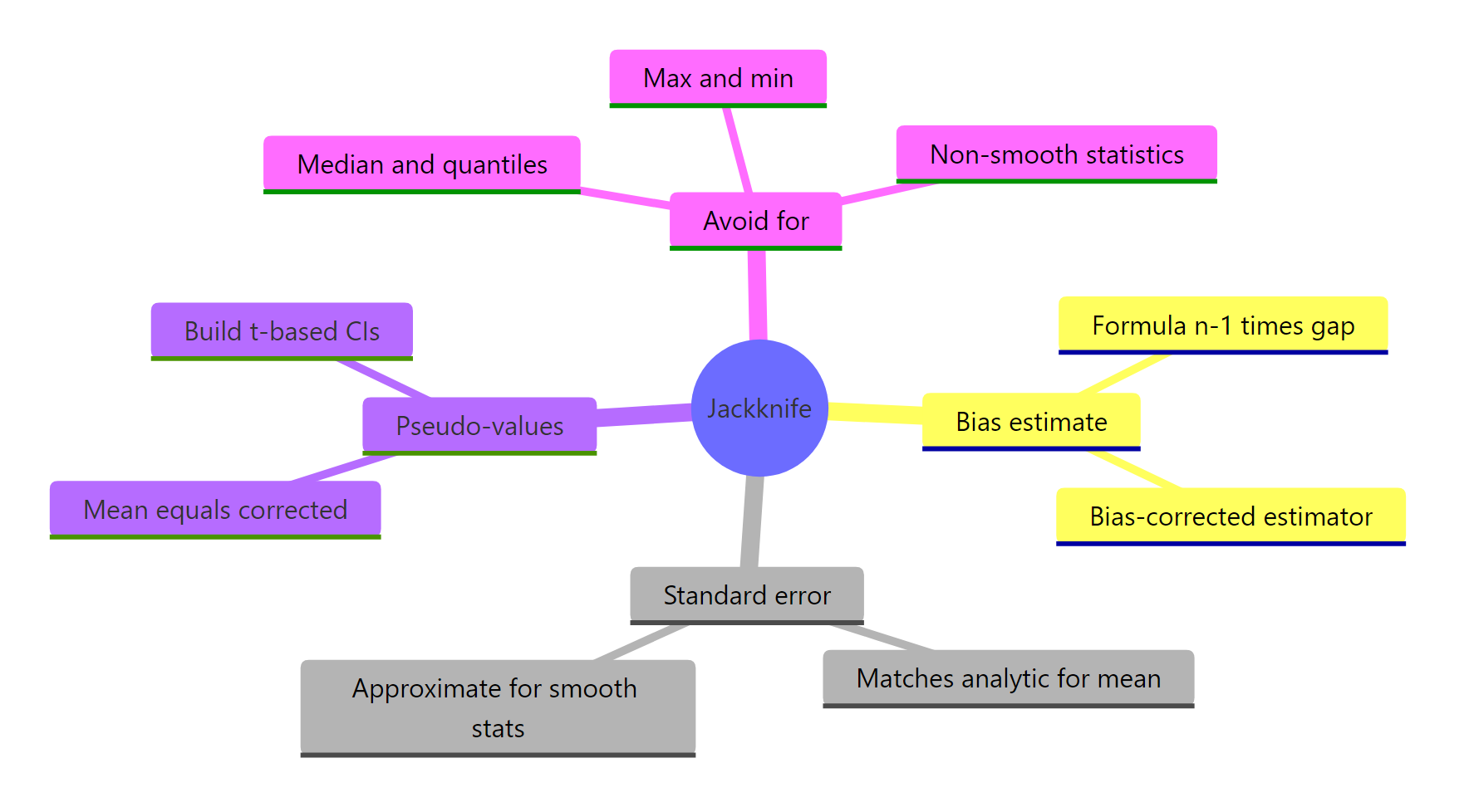
Figure 2: What the jackknife gives you, and where it falls short.

What you want	Jackknife formula
Standard error	$\sqrt{\frac{n-1}{n}\sum (\hat\theta_{(-i)} - \bar\theta_\text{jack})^2}$
Bias estimate	$(n-1)(\bar\theta_\text{jack} - \hat\theta)$
Bias-corrected estimate	$n\hat\theta - (n-1)\bar\theta_\text{jack}$
Pseudo-value	$\varphi_i = n\hat\theta - (n-1)\hat\theta_{(-i)}$
Confidence interval	$\bar\varphi \pm t_{n-1,\alpha/2} \cdot \mathrm{sd}(\varphi)/\sqrt{n}$

Use the jackknife when your statistic is smooth (means, ratios, regression coefficients, correlations, log-likelihoods). Reach for the bootstrap when it is not (medians, quantiles, max, min, anything with a min/max/sort step in the middle).

References

Quenouille, M.H. (1949). Approximate tests of correlation in time series. Journal of the Royal Statistical Society B, 11, 68-84.
Tukey, J.W. (1958). Bias and confidence in not-quite large samples (abstract). Annals of Mathematical Statistics, 29, 614.
Efron, B., Tibshirani, R.J. (1993). An Introduction to the Bootstrap. Chapman & Hall, ch. 11.
Shalizi, C. (2023). Jackknife notes, CMU Stat 36-490. Link
Wikipedia: Jackknife resampling. Link
Zivot, E. Introduction to Computational Finance and Financial Econometrics with R, ch. 8.5. Link
Sawyer, S. (2005). Resampling Data: Using a Statistical Jackknife. Washington University. Link
Joanes, D.N., Gill, C.A. (1998). Comparing measures of sample skewness and kurtosis. Journal of the Royal Statistical Society D, 47(1), 183-189.

Continue Learning

Bootstrap in R, the resampling sibling that handles non-smooth statistics where the jackknife fails.
Bootstrap Confidence Intervals in R, for when the t-CI on pseudo-values is not enough and you need percentile or BCa intervals.
When to Use Nonparametric Tests in R, the broader nonparametric toolkit that resampling methods sit inside.

Jackknife Resampling in R: Leave-One-Out Bias Correction

What is jackknife resampling, and how does it work?

How do you estimate bias with the jackknife?

How do you compute the jackknife standard error and confidence intervals?

When does the jackknife fail (and what to use instead)?

Practice Exercises

Exercise 1: Trimmed-mean SE on airquality

Exercise 2: A reusable jackknife CI function

Exercise 3: Influential observations from pseudo-values

Complete Example

Summary

References

Continue Learning

Related Tutorials