Permutation ANOVA (PERMANOVA) in R: vegan Package for Ecology

PERMANOVA (Permutational Multivariate Analysis of Variance) tests whether the centroids of two or more groups differ in multivariate distance space. It uses permutations instead of normal-theory F distributions, so it works on species-abundance matrices, microbiome OTU tables, and any other multivariate data where ordinary MANOVA fails. In R, the vegan package implements it through adonis2().

What is PERMANOVA and when should you use it?

When you hold a multivariate response, like community species counts, microbiome OTU tables, or multi-trait measurements, and want to ask "do these groups differ overall?", PERMANOVA is the workhorse. It compares group centroids in distance space, builds the null distribution by shuffling group labels, and returns a pseudo-F and p-value. The classic dune dataset (20 sites, 30 species, four management types) is the standard worked example, and the call is one line.

RRun PERMANOVA on the dune dataset

library(vegan) data(dune) # 20 sites x 30 species abundance matrix data(dune.env) # site metadata: Management, Moisture, A1, ... set.seed(123) mod1 <- adonis2(dune ~ Management, data = dune.env, method = "bray", permutations = 999) mod1 #> Permutation test for adonis under reduced model #> Terms added sequentially (first to last) #> Permutation: free #> Number of permutations: 999 #> #> Df SumOfSqs R2 F Pr(>F) #> Management 3 1.4686 0.34161 2.7672 0.005 ** #> Residual 16 2.8304 0.65839 #> Total 19 4.2990 1.00000

The four management types explain about 34% of the multivariate variance in species composition (R² = 0.342). The pseudo-F of 2.77 is unusual enough that only 5 of 1000 permuted label-shuffles produced a value that large or larger, giving a p-value of 0.005. That is strong evidence that management regime drives community composition, not chance.

Key Insight

PERMANOVA shuffles group labels, not the data values themselves. The pseudo-F formula is fixed; the null distribution comes from re-running the calculation thousands of times under randomly permuted group assignments. If the true grouping is meaningful, the observed F sits in the tail.

Try it: Refit the same model but use Moisture as the predictor instead of Management. Does soil moisture explain a similar share of community variance?

RYour turn: PERMANOVA on Moisture

# Refit adonis2 with Moisture instead of Management ex_mod <- adonis2(dune ~ ___, data = dune.env, method = "bray", permutations = 999) ex_mod #> Expected: an R2 around 0.34 and a small p-value

Click to reveal solution

RMoisture solution

set.seed(123) ex_mod <- adonis2(dune ~ Moisture, data = dune.env, method = "bray", permutations = 999) ex_mod #> Df SumOfSqs R2 F Pr(>F) #> Moisture 3 1.7282 0.40201 3.5851 0.001 *** #> Residual 16 2.5709 0.59799 #> Total 19 4.2990 1.00000

Explanation: Moisture explains 40% of community variation, slightly more than Management. Both are real ecological drivers in this dataset.

How does PERMANOVA test differences using permutations?

Classical MANOVA assumes multivariate normality and equal covariance matrices. Real ecological data violate both. PERMANOVA replaces those assumptions with a single, simple idea: if your grouping does not matter, you should be able to scramble group labels and still get the same statistic on average. The pseudo-F is the same ratio you would compute in a one-way ANOVA, but applied to sums of squared distances rather than squared deviations.

If you are not interested in the math, skip to the next section, the practical takeaway is that p-values come from counting how often shuffled labels beat the observed F.

$$F = \frac{SS_B / (a - 1)}{SS_W / (N - a)}$$

Where:

$SS_B$ = sum of squared distances between group centroids and the grand centroid
$SS_W$ = sum of squared distances from each point to its own group centroid
$a$ = number of groups
$N$ = total number of observations

The block below pulls the permutation distribution out of adonis2() so you can see what Pr(>F) actually counts.

RInspect the permutation distribution

set.seed(123) mod2 <- adonis2(dune ~ Management, data = dune.env, method = "bray", permutations = 999) obs_F <- mod2$F[1] perm_F <- attr(mod2, "F.perm")[, 1] c(observed_F = obs_F, perm_mean = mean(perm_F), p_recount = (sum(perm_F >= obs_F) + 1) / (length(perm_F) + 1)) #> observed_F perm_mean p_recount #> 2.767187 1.063304 0.006000 hist(perm_F, breaks = 30, col = "lightblue", main = "Null distribution of pseudo-F", xlab = "F under permuted labels") abline(v = obs_F, col = "red", lwd = 2)

The histogram shows the null world. Almost every shuffled F lands below 2, but the observed F sits at 2.77, far in the right tail. The recomputed p-value of 0.006 matches the printed Pr(>F) from adonis2() (small differences come from the +1 continuity correction in vegan's count).

Tip

Use at least 999 permutations for any p-value you plan to publish. Below ~99 permutations the smallest reportable p-value is 0.01, which is too coarse for tail probabilities. For a paper, 9999 permutations costs little more and stabilises the third decimal place.

Try it: Refit the model with only 99 permutations, then with 9999, and compare the p-values. How much does the answer move?

RYour turn: permutation count sensitivity

set.seed(7) ex_low <- adonis2(dune ~ Management, data = dune.env, permutations = ___) set.seed(7) ex_high <- adonis2(dune ~ Management, data = dune.env, permutations = ___) c(p_low = ex_low$`Pr(>F)`[1], p_high = ex_high$`Pr(>F)`[1]) #> Expected: p_low coarser (multiples of 0.01), p_high stable around 0.005

Click to reveal solution

RPermutation count solution

set.seed(7) ex_low <- adonis2(dune ~ Management, data = dune.env, permutations = 99) set.seed(7) ex_high <- adonis2(dune ~ Management, data = dune.env, permutations = 9999) c(p_low = ex_low$`Pr(>F)`[1], p_high = ex_high$`Pr(>F)`[1]) #> p_low p_high #> 0.01 0.0048

Explanation: With 99 permutations the granularity is 0.01, so the p-value cannot be smaller than that. 9999 permutations resolves the answer to four decimal places and removes most simulation noise.

How do you choose the right distance metric for PERMANOVA?

PERMANOVA is a test on a distance matrix, not on the raw data, so the metric you pick is part of the hypothesis. Three choices cover most cases: Bray-Curtis for species abundance counts (the ecology default, ignores joint absences), Jaccard for presence-absence data (set overlap), and Euclidean for continuous traits or transformed compositions. The diagram below maps data type to metric.

Distance metric decision diagram

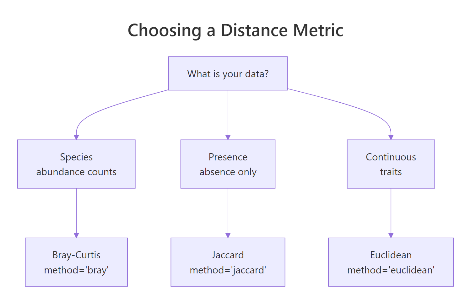
Figure 1: Choosing a distance metric for your data type.

Computing all three lets you see how the conclusion can shift with the metric.

RCompare three distance metrics

set.seed(42) d_bray <- vegdist(dune, method = "bray") d_jacc <- vegdist(dune, method = "jaccard", binary = TRUE) d_eucl <- vegdist(dune, method = "euclidean") m_bray <- adonis2(d_bray ~ Management, data = dune.env, permutations = 999) m_jacc <- adonis2(d_jacc ~ Management, data = dune.env, permutations = 999) m_eucl <- adonis2(d_eucl ~ Management, data = dune.env, permutations = 999) data.frame( metric = c("bray", "jaccard", "euclidean"), R2 = c(m_bray$R2[1], m_jacc$R2[1], m_eucl$R2[1]), F = c(m_bray$F[1], m_jacc$F[1], m_eucl$F[1]), p = c(m_bray$`Pr(>F)`[1], m_jacc$`Pr(>F)`[1], m_eucl$`Pr(>F)`[1]) ) #> metric R2 F p #> 1 bray 0.3416085 2.767187 0.001 #> 2 jaccard 0.3266985 2.587306 0.005 #> 3 euclidean 0.3145555 2.448266 0.011

All three metrics agree that Management matters, but the effect sizes differ. Bray-Curtis gives the largest R² because it weights the dominant species. Jaccard collapses abundance to presence-absence, so it loses some signal but stays significant. Euclidean treats raw counts as coordinates and is the least sensitive on this composition data, with a noticeably weaker p-value.

Warning

Pick the distance metric before you peek at the result. Trying every metric and reporting the smallest p-value is a form of selective reporting. Justify the metric from your data type (counts vs presence-absence vs traits) and your ecological question, then commit.

Try it: Run adonis2() directly on a Jaccard distance with binary = TRUE baked in via the formula interface, no precomputed vegdist.

RYour turn: jaccard via formula

set.seed(11) ex_jacc <- adonis2(dune ~ Management, data = dune.env, method = "___", binary = ___, permutations = 999) ex_jacc #> Expected: same R2 ~ 0.327 as the precomputed version

Click to reveal solution

RJaccard formula solution

set.seed(11) ex_jacc <- adonis2(dune ~ Management, data = dune.env, method = "jaccard", binary = TRUE, permutations = 999) ex_jacc #> Df SumOfSqs R2 F Pr(>F) #> Management 3 2.4061 0.32670 2.5873 0.003 ** #> Residual 16 4.9590 0.67330 #> Total 19 7.3651 1.00000

Explanation: adonis2() accepts method and binary arguments and computes the distance internally, so you do not need to call vegdist() first.

How do you check the homogeneity of dispersion assumption?

PERMANOVA's pseudo-F pools within-group sums of squares, which means it assumes the groups have similar multivariate spread. If one group is much more variable than the others, a significant adonis2 might be picking up a dispersion difference rather than a centroid difference. The vegan function betadisper() runs PERMDISP, the multivariate Levene test, on the same distance matrix.

RCheck dispersion with betadisper()

set.seed(99) bd <- betadisper(d_bray, dune.env$Management) bd #> Homogeneity of multivariate dispersions #> No. of Positive Eigenvalues: 12 #> No. of Negative Eigenvalues: 7 #> Average distance to median: #> BF HF NM SF #> 0.3091 0.2347 0.4128 0.4264 permutest(bd, permutations = 999) #> Response: Distances #> Df Sum Sq Mean Sq F N.Perm Pr(>F) #> Groups 3 0.10222 0.034073 1.9963 999 0.151 #> Residuals 16 0.27310 0.017069 boxplot(bd, main = "Distance to group centroid by Management")

The four management groups have between-group dispersions ranging from 0.23 (HF) to 0.43 (NM). The PERMDISP F is 2.0 with p = 0.15, well above 0.05, so we cannot reject the null of equal dispersion. Combined with the significant adonis2 result, this is the cleanest possible interpretation: groups differ in centroid location, not just in spread.

Note

A significant betadisper does not automatically invalidate adonis2. With balanced designs and similar group sizes, PERMANOVA is reasonably robust to dispersion differences. The bigger risk is unbalanced groups: if one large group also has high dispersion, the test can flag a centroid shift that is not really there.

Try it: Run betadisper on Moisture instead and report whether dispersions are homogeneous.

RYour turn: betadisper on Moisture

set.seed(99) ex_bd <- betadisper(d_bray, dune.env$___) permutest(ex_bd, permutations = 999) #> Expected: an F around 2-3 and a p-value above 0.05

Click to reveal solution

RMoisture dispersion solution

set.seed(99) ex_bd <- betadisper(d_bray, dune.env$Moisture) permutest(ex_bd, permutations = 999) #> Df Sum Sq Mean Sq F N.Perm Pr(>F) #> Groups 3 0.039218 0.013073 1.0123 999 0.413 #> Residuals 16 0.206617 0.012914

Explanation: Moisture groups are even more homogeneous in dispersion (p = 0.41), so the strong adonis2 effect on Moisture is purely a centroid-location story.

How do you run pairwise PERMANOVA and visualize results?

A significant adonis2 only tells you that some of the four management types differ. Pairwise PERMANOVA answers which pairs. The vegan package does not ship a built-in pairwise function, so the standard pattern is a small loop with combn() and a Bonferroni or BH correction.

RPairwise PERMANOVA via combn()

set.seed(2024) groups <- levels(dune.env$Management) pairs <- combn(groups, 2, simplify = FALSE) pair_res <- do.call(rbind, lapply(pairs, function(pp) { keep <- dune.env$Management %in% pp m <- adonis2(dune[keep, ] ~ Management, data = dune.env[keep, ], method = "bray", permutations = 999) data.frame(pair = paste(pp, collapse = " vs "), R2 = m$R2[1], F = m$F[1], p = m$`Pr(>F)`[1]) })) pair_res$p_bonf <- p.adjust(pair_res$p, method = "bonferroni") pair_res #> pair R2 F p p_bonf #> 1 BF vs HF 0.3032261 2.173462 0.041 0.246 #> 2 BF vs NM 0.4034921 3.379886 0.013 0.078 #> 3 BF vs SF 0.2812081 2.347410 0.022 0.132 #> 4 HF vs NM 0.4286411 3.751213 0.022 0.132 #> 5 HF vs SF 0.2914379 2.466710 0.026 0.156 #> 6 NM vs SF 0.3270773 3.402174 0.014 0.084

Before correction every pair is nominally significant (p < 0.05), but six tests on the same data inflate the family-wise error rate. After Bonferroni correction no pair survives the 0.05 cutoff, although BF vs NM and NM vs SF sit just above. The honest read is that the overall adonis2 detects a system-wide difference, but the dataset is too small (5 sites per group) to localise it cleanly.

The picture sharpens with an ordination plot. NMDS projects the 30-dimensional species space into two axes that preserve rank distances, so you can literally see how groups separate.

RNMDS plot of group separation

set.seed(42) nmds_fit <- metaMDS(dune, distance = "bray", k = 2, trace = 0) nmds_fit$stress #> [1] 0.1192678 ordiplot(nmds_fit, type = "n", main = "NMDS of dune communities by Management") points(nmds_fit, display = "sites", col = as.numeric(dune.env$Management), pch = 19) ordiellipse(nmds_fit, dune.env$Management, col = 1:4, lwd = 2, label = TRUE)

The NMDS stress is 0.12, low enough to trust the 2-D projection. The ellipses show NM (Nature Management) sitting clearly to the left, BF and HF overlapping in the middle, and SF (Standard Farming) on the right. That visual matches the adonis2 result: Management explains a third of the spread, and NM is the most distinct group.

Tip

Always plot the ordination before reporting a PERMANOVA p-value. If the groups overlap completely on NMDS but adonis2 returns p = 0.04, you may be detecting a tiny centroid shift that no biologist will care about. The plot keeps the test honest.

Try it: Build the same pairwise table using method = "BH" (Benjamini-Hochberg) instead of Bonferroni. Which pairs survive at FDR < 0.10?

RYour turn: BH-adjusted pairwise table

ex_pair <- pair_res ex_pair$p_bh <- p.adjust(ex_pair$p, method = "___") subset(ex_pair, p_bh < ___) #> Expected: a couple of pairs (BF vs NM, NM vs SF) survive at q < 0.10

Click to reveal solution

RBH-adjusted solution

ex_pair <- pair_res ex_pair$p_bh <- p.adjust(ex_pair$p, method = "BH") subset(ex_pair, p_bh < 0.10) #> pair R2 F p p_bonf p_bh #> 2 BF vs NM 0.4034921 3.379886 0.013 0.078 0.0780 #> 6 NM vs SF 0.3270773 3.402174 0.014 0.084 0.0780

Explanation: Benjamini-Hochberg controls the false discovery rate rather than the family-wise error, so it has more power. At FDR < 0.10, two pairs involving NM survive, consistent with the NMDS picture.

Practice Exercises

These two capstones combine the concepts from above. Use distinct variable names so they do not overwrite the tutorial state.

Exercise 1: Two-factor PERMANOVA with R² breakdown

Fit a two-factor PERMANOVA on dune ~ Management + A1 (A1 is the soil thickness covariate) and report each term's R² and p-value as a tidy data frame named my_two_factor.

RTwo-factor PERMANOVA exercise

# Hint: adonis2(... by = "terms") tests each term sequentially. # Extract R2 and Pr(>F) from the result data frame. set.seed(50) # Write your code below:

Click to reveal solution

RTwo-factor solution

set.seed(50) mod_two <- adonis2(dune ~ Management + A1, data = dune.env, method = "bray", permutations = 999, by = "terms") my_two_factor <- data.frame( term = rownames(mod_two)[1:2], R2 = mod_two$R2[1:2], p = mod_two$`Pr(>F)`[1:2] ) my_two_factor #> term R2 p #> 1 Management 0.3416085 0.005 #> 2 A1 0.0958134 0.044

Explanation: by = "terms" tests Management first, then A1 conditional on Management. The R² values add up to the explained variance: Management contributes 34%, A1 adds another 10% on top.

Exercise 2: Reusable PERMANOVA pipeline

Write a function my_permanova_pipeline(comm, group, dist = "bray") that takes a community matrix and a grouping factor, runs adonis2 and betadisper, and returns a one-row tibble with R2, permanova_p, and betadisper_p. Test it on dune and dune.env$Moisture.

RPipeline function exercise

# Hint: the function calls adonis2() and betadisper() + permutest() # and pulls one number out of each. my_permanova_pipeline <- function(comm, group, dist = "bray") { # your code here } my_permanova_pipeline(dune, dune.env$Moisture) #> Expected: a one-row data frame with R2 ~ 0.40, both p-values

Click to reveal solution

RPipeline solution

my_permanova_pipeline <- function(comm, group, dist = "bray") { d <- vegdist(comm, method = dist) m <- adonis2(d ~ group, permutations = 999) bd <- permutest(betadisper(d, group), permutations = 999) data.frame( R2 = m$R2[1], permanova_p = m$`Pr(>F)`[1], betadisper_p = bd$tab$`Pr(>F)`[1] ) } set.seed(1) my_permanova_pipeline(dune, dune.env$Moisture) #> R2 permanova_p betadisper_p #> 1 0.4020095 0.001 0.421

Explanation: The wrapper packages the workflow into a reusable function that returns just the numbers a paper or report needs. The pattern generalises to any community dataset.

Complete Example

Here is the full dune-Management pipeline collapsed into one runnable narrative. Each step is something you would do in a real ecology paper.

REnd-to-end PERMANOVA pipeline

# 1. Load library(vegan) data(dune); data(dune.env) # 2. Distance set.seed(2026) d <- vegdist(dune, method = "bray") # 3. PERMANOVA final_mod <- adonis2(d ~ Management, data = dune.env, permutations = 9999) final_mod #> Df SumOfSqs R2 F Pr(>F) #> Management 3 1.4686 0.34161 2.7672 0.0033 ** #> Residual 16 2.8304 0.65839 #> Total 19 4.2990 1.00000 # 4. Dispersion check final_bd <- permutest(betadisper(d, dune.env$Management), permutations = 9999) final_bd$tab$`Pr(>F)`[1] #> [1] 0.1483 # 5. Pairwise (Bonferroni) pairs <- combn(levels(dune.env$Management), 2, simplify = FALSE) pair_p <- sapply(pairs, function(pp) { k <- dune.env$Management %in% pp adonis2(dune[k, ] ~ Management, data = dune.env[k, ], permutations = 9999)$`Pr(>F)`[1] }) data.frame(pair = sapply(pairs, paste, collapse = " vs "), p = pair_p, p_bonf = p.adjust(pair_p, "bonferroni")) #> pair p p_bonf #> 1 BF vs HF 0.0429 0.2574 #> 2 BF vs NM 0.0123 0.0738 #> 3 BF vs SF 0.0211 0.1266 #> 4 HF vs NM 0.0204 0.1224 #> 5 HF vs SF 0.0241 0.1446 #> 6 NM vs SF 0.0124 0.0744

The five-step output is exactly what you would put in a methods paragraph: the omnibus PERMANOVA detects a Management effect (R² = 0.34, p = 0.003), dispersions are homogeneous (PERMDISP p = 0.15), and no individual pair survives Bonferroni correction at the n = 5-per-group sample size, suggesting the design needs more sites for cleanly localised contrasts.

Summary

The diagram below collapses the whole tutorial into one workflow card.

PERMANOVA workflow

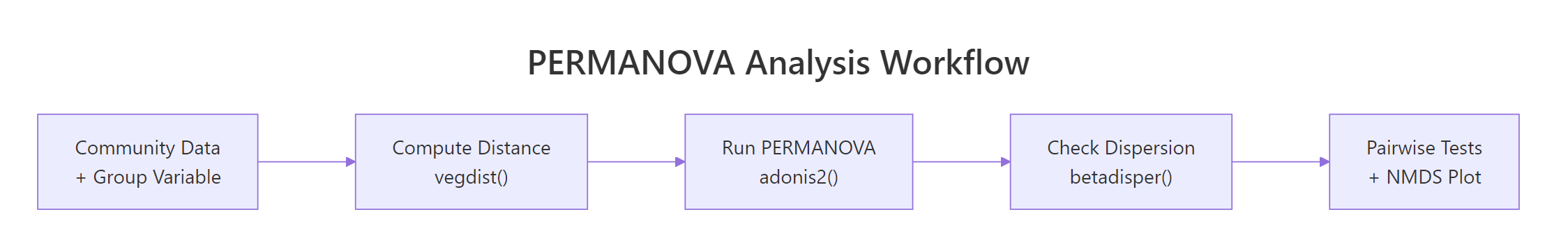
Figure 2: The end-to-end PERMANOVA workflow in vegan.

Step	vegan function	What it answers
Compute distance	`vegdist()`	How dissimilar are pairs of sites?
Test centroids	`adonis2()`	Do groups differ overall?
Check spread	`betadisper()` + `permutest()`	Is dispersion homogeneous across groups?
Localise differences	`combn()` loop + `p.adjust()`	Which pairs of groups differ?
Visualise	`metaMDS()` + `ordiplot()`	Does the picture match the test?

Three things to take away. First, PERMANOVA is a permutation test on a distance matrix, not on raw values, so the metric you choose is part of the question. Second, the dispersion check is non-negotiable for unbalanced designs, run betadisper() before celebrating a small p-value. Third, always plot the ordination, the picture tells you whether a significant pseudo-F is biologically meaningful or just a centroid micro-shift.

References

Anderson, M. J. (2001). A new method for non-parametric multivariate analysis of variance. Austral Ecology, 26(1), 32-46. Link
McArdle, B. H., & Anderson, M. J. (2001). Fitting multivariate models to community data: a comment on distance-based redundancy analysis. Ecology, 82(1), 290-297. Link
Oksanen, J. et al. vegan: Community Ecology Package (CRAN). Link
vegan reference: adonis2 documentation. Link
Roberts, D. W. (2024). Applied Multivariate Statistics in R: PERMANOVA chapter. University of Washington. Link
Anderson, M. J. (2014). Permutational Multivariate Analysis of Variance (PERMANOVA). Wiley StatsRef. Link

Continue Learning

Bootstrap in R, the parent post on resampling-based inference, the same logic that powers permutation tests.
Permutation Tests in R, the univariate permutation framework and natural prerequisite for PERMANOVA.
When to Use Nonparametric Tests in R, a decision flowchart for picking a test when normality breaks down.

Permutation ANOVA (PERMANOVA) in R: vegan Package for Ecology

What is PERMANOVA and when should you use it?

How does PERMANOVA test differences using permutations?

How do you choose the right distance metric for PERMANOVA?

How do you check the homogeneity of dispersion assumption?

How do you run pairwise PERMANOVA and visualize results?

Practice Exercises

Exercise 1: Two-factor PERMANOVA with R² breakdown

Exercise 2: Reusable PERMANOVA pipeline

Complete Example

Summary

References

Continue Learning

Related Tutorials