Anderson-Darling Test in R: Sensitive Normality Test Alternative
The Anderson-Darling test in R checks whether a sample comes from a specified distribution, most often the Normal. Run it with nortest::ad.test(x): the function returns an A statistic that weights deviations in the tails more heavily than Shapiro-Wilk or Kolmogorov-Smirnov, plus a p-value testing the null hypothesis that the data are normally distributed.
When you have outliers, fat tails, or you care about the extremes of your distribution, the Anderson-Darling test will catch the problem when other normality tests miss it. That tail sensitivity is the whole reason it exists.
How do you run the Anderson-Darling test in R?
You have a numeric vector and you want to know whether it is normally distributed before fitting a t-test, a regression, or an ANOVA. The Anderson-Darling test answers that with one function call from the nortest package. Generate a sample from a known Normal, run ad.test(), and read off A and the p-value.
A is 0.214: a small value because the empirical distribution closely matches a Normal across the whole range. The p-value of 0.84 is far above the conventional 0.05 threshold, so we fail to reject the null hypothesis. The data look Normal, which is exactly what we would hope for a sample drawn from rnorm().
shapiro.test() in most analysis pipelines.Try it: Run ad.test() on a sample of 50 values from a Normal with mean 10 and sd 2. Save the result to ex_result1 and print it.
Click to reveal solution
Explanation: The mean and sd are estimated internally, so shifting the location or rescaling does not change the verdict. The data still look Normal.
What does the A statistic actually measure?
The Anderson-Darling statistic measures how far the empirical cumulative distribution function (ECDF) of your data is from the theoretical Normal CDF. The trick is in the weighting: it gives much more weight to the tails of the distribution than to the middle. That is why it catches outliers and heavy tails that other tests overlook.
The formula looks like this:
$$A^2 = -n - \sum_{i=1}^{n} \frac{2i-1}{n} \left[ \ln F(x_{(i)}) + \ln(1 - F(x_{(n+1-i)})) \right]$$
Where:
- $n$ = sample size
- $x_{(i)}$ = the $i$-th order statistic (sorted data)
- $F(\cdot)$ = the theoretical CDF (the Normal CDF here)
- The $\ln F$ and $\ln(1-F)$ terms blow up when $F$ is near 0 or 1, which is exactly the tail region
If you are not interested in the math, skip to the next code block. The practical R code is all you need.
To see the tail sensitivity in action, compare a clean Normal sample with a t-distributed sample. The t with low degrees of freedom has the same bell shape near the centre but much heavier tails.
The Normal sample gives A = 0.21, while the heavy-tailed t sample gives A = 1.55, more than seven times larger. The middle of the t distribution looks roughly bell-shaped, but the extreme observations push A up sharply because the tail weighting amplifies them. Shapiro-Wilk and KS would also flag this, but the AD signal is loudest.
Try it: Compute ad.test() on a sample of 80 values from a t-distribution with 4 degrees of freedom. Look at the A statistic.
Click to reveal solution
Explanation: With df=4 the tails are heavier than Normal but lighter than df=3. A lands between the two, and the p-value of 0.008 rejects normality at the 0.01 level.
How does Anderson-Darling compare to Shapiro-Wilk and Kolmogorov-Smirnov?
R gives you three popular normality tests: shapiro.test() from base R, ks.test() from base R, and nortest::ad.test(). Each has different strengths. Run all three on the same Normal sample to see how their p-values line up under the null.
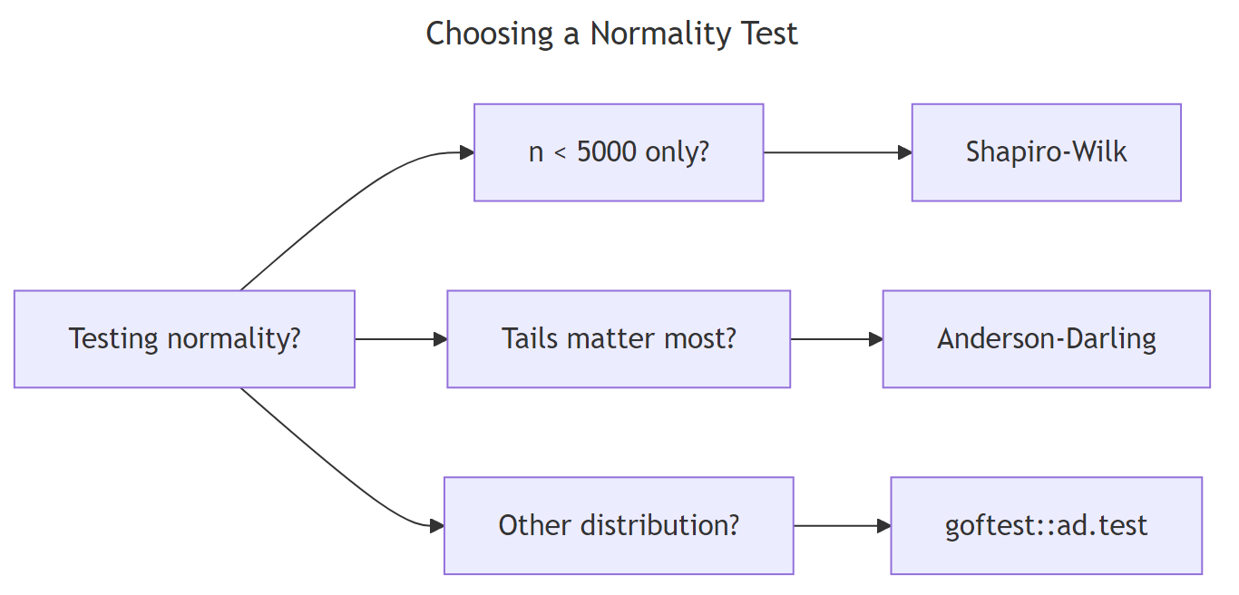
Figure 1: Choosing among Anderson-Darling, Shapiro-Wilk, and Kolmogorov-Smirnov by question.
All three p-values are large, as expected for a true Normal sample, and the three methods broadly agree. The interesting differences appear when the data is not Normal. Try the same comparison on Cauchy-distributed data, which has tails so heavy the variance is undefined.
All three reject normality, but Anderson-Darling delivers the smallest p-value by orders of magnitude, while KS is least decisive. That gap reflects the tail weighting: the few extreme Cauchy observations dominate the AD statistic, while KS only sees the worst-case gap and downweights extremes.
nortest::lillie.test() (Lilliefors correction) or ad.test() instead.Try it: Run all three tests on rnorm(60) and on rcauchy(60). Which test gives the strongest signal each time?
Click to reveal solution
Explanation: On Normal data both tests give large p-values. On Cauchy, AD typically gives a smaller p-value than SW because of its tail weighting.
How do you test fit to non-normal distributions?
nortest::ad.test() only tests fit to the Normal. To check whether your data fit an exponential, gamma, or any other continuous distribution, use goftest::ad.test(), which accepts an arbitrary CDF function and its parameters.
The p-value of 0.90 is large, so we fail to reject the null that the sample comes from an Exp(0.5) distribution. The function works the same way for any CDF: pass "pgamma", "plnorm", "pweibull", or your own CDF function in the null argument and supply the parameters.
goftest::ad.test() with estimated = TRUE if available, or nortest's special-case tests (ad.test, cvm.test, lillie.test) for the Normal.Try it: Test whether a sample from rgamma(100, shape = 2, rate = 1) fits a Gamma(2, 1) distribution.
Click to reveal solution
Explanation: Pass the CDF name ("pgamma") and its parameters as named arguments. The test returns An (the AD statistic adapted for arbitrary distributions) and a p-value.
When does the Anderson-Darling test fail or mislead you?
Three situations trip up Anderson-Darling. First, very small samples (n < 8) leave too little tail data to weight, and the test loses power. Second, ties in continuous data (caused by rounding) violate the test's assumptions. Third, with very large n, even tiny departures from Normal become "significant" because the test is too powerful for its own good.
The data is 98% Normal with a 2% mixture component shifted by 0.5, which is invisible on a histogram. With n = 10000 the AD test rejects normality with a p-value below 2.2e-16. Mathematically true, practically useless: a t-test or regression would be perfectly fine on this data.
n > 1000, supplement any normality test with a Q-Q plot. Use the test as a sanity check, not a verdict.Try it: Run ad.test() on rnorm(50) and on rnorm(5000). Compare the A statistics.
Click to reveal solution
Explanation: The A statistic is roughly the same scale because both samples are truly Normal. Both p-values will be large. The lesson is that A itself is comparable across sample sizes; the p-value is what shifts when n grows.
Practice Exercises
Exercise 1: Diagnose three samples in one pipeline
Simulate three samples of size 100 each from a Normal(0,1), Exponential(1), and t with 3 degrees of freedom. Build a data frame with columns sample, A, and p_value, sorted by p_value ascending. Save it to my_diag.
Click to reveal solution
Explanation: The Exponential has the strongest signal, t with df=3 also rejects, and the Normal sample passes. Sorting by p-value gives a quick visual diagnosis.
Exercise 2: Build a verdict function
Write a function ad_diagnose(x) that runs ad.test() and returns a named list with A, p, and a one-word verdict: "normal" if p > 0.05, "reject" otherwise. Test it on rnorm(80) and rt(80, df = 2).
Click to reveal solution
Explanation: Wrapping a test in a tiny diagnostic function pays off when you run it across many groups in a real workflow.
Complete Example
Here is the full workflow you would actually run on real data: test for normality, transform if rejected, re-test, and confirm with a Q-Q plot.
The raw mpg p-value of 0.12 is borderline; after a log transform it rises to 0.34, and the Q-Q plot of log(mpg) hugs the diagonal more tightly. For downstream regression on a small dataset like mtcars, the log scale is the safer choice.
Summary
| Aspect | Anderson-Darling | Shapiro-Wilk | Kolmogorov-Smirnov |
|---|---|---|---|
| Function | nortest::ad.test() |
shapiro.test() |
ks.test() |
| Best n range | 8 to 5000 | 3 to 5000 | any size |
| Tail sensitivity | high | medium | low |
| Tests other distributions | yes (goftest::ad.test) |
no | yes |
| Estimated parameters OK | yes | yes | no (use Lilliefors) |
| Power on heavy tails | best | good | weakest |
Use Anderson-Darling when you suspect heavy tails or care about extreme values. Use Shapiro-Wilk for the gold-standard small-sample normality check. Use KS only when the distribution and its parameters are fully specified up front.
References
- Anderson, T. W. and Darling, D. A. (1952). Asymptotic theory of certain "goodness-of-fit" criteria based on stochastic processes. Annals of Mathematical Statistics, 23, 193-212. Link
- Gross, J. and Ligges, U., nortest package documentation. Link
- Faraway, J., Marsaglia, G., Marsaglia, J. and Baddeley, A., goftest package documentation. Link
- NIST/SEMATECH e-Handbook of Statistical Methods, Anderson-Darling test. Link
- Razali, N. M. and Wah, Y. B. (2011). Power comparisons of Shapiro-Wilk, Kolmogorov-Smirnov, Lilliefors and Anderson-Darling tests. Journal of Statistical Modeling and Analytics, 2, 21-33.
- Stephens, M. A. (1974). EDF statistics for goodness of fit and some comparisons. Journal of the American Statistical Association, 69, 730-737.
Continue Learning
- When to Use Nonparametric Tests in R, the parent guide on choosing nonparametric methods
- Kolmogorov-Smirnov Two-Sample Test in R, compare two distributions without assuming Normal
- Wilcoxon Signed-Rank Test in R, when normality fails and you need a one-sample location test