Segmented Regression in R: Breakpoints, Piecewise Linear & Threshold

Segmented regression fits two or more straight lines joined at estimated breakpoints, ideal when a relationship changes slope abruptly rather than curving smoothly. In R, the segmented package estimates the breakpoint, the slope on each side, and a confidence interval for the join itself, starting from any lm() you already have.

When should you use segmented regression instead of polynomial or spline?

A scatter plot that bends is not the same as a scatter plot that kinks. A bend is smooth curvature, a kink is an abrupt change of slope at a specific x. Polynomial and spline regression fit the first cleanly; they wobble through a kink and leave systematic residuals. Segmented regression assumes the kink, estimates where it sits, and returns one slope per regime. The payoff below shows the difference on a simulated dose-response with a threshold at x = 30.

RFit segmented model to threshold data

# Load libraries used throughout the tutorial library(segmented) library(ggplot2) # Simulate dose-response with a kink at x = 30 set.seed(2024) x <- runif(120, 0, 60) y <- 0.2 * x + ifelse(x > 30, 0.8 * (x - 30), 0) + rnorm(120, sd = 1.5) df_kink <- data.frame(x = x, y = y) # Fit base linear model, then add a single breakpoint fit_lin <- lm(y ~ x, data = df_kink) fit_seg <- segmented(fit_lin, seg.Z = ~ x, psi = 25) # Compare the estimated breakpoint to the true value of 30 summary(fit_seg)$psi #> Initial Est. St.Err #> psi1.x 25 29.85 0.481

The algorithm refined our starting guess of 25 to a breakpoint of 29.85, within 0.15 of the true value of 30, and the standard error of 0.481 says the location is pinned tight. A linear fit would have split the difference between the two regimes and smeared the slope change across the whole range.

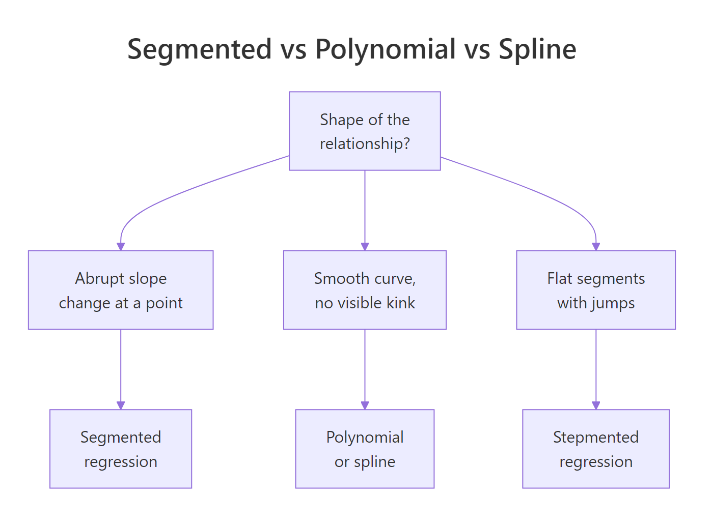
When segmented regression fits better than polynomial or spline.

Figure 1: When segmented regression fits better than polynomial or spline.

Key Insight

Segmented regression assumes the kink; polynomial and spline regression discover curves. If you know the relationship changes at some point but not which point, segmented regression is designed for you. If you only know the shape is not a straight line, a spline is safer because it does not commit to a kink that might not exist.

Try it: Fit a 2-segment model to the built-in cars dataset with starting breakpoint psi = 15, then print the estimated breakpoint. The cars data relates dist (stopping distance) to speed (mph) for 50 cars.

RYour turn: fit segmented model to cars

# Fit a base lm, then segmented() ex_fit_base <- lm(dist ~ speed, data = cars) ex_fit_seg <- # your code here # Print the estimated breakpoint # Expected: a psi estimate roughly in the 12-18 mph range

Click to reveal solution

RSegmented model on cars solution

ex_fit_base <- lm(dist ~ speed, data = cars) ex_fit_seg <- segmented(ex_fit_base, seg.Z = ~ speed, psi = 15) summary(ex_fit_seg)$psi #> Initial Est. St.Err #> psi1.speed 15 17.586 2.26

Explanation: The estimated breakpoint near 17.6 mph matches the bend in cars, where stopping distance grows faster with speed at higher speeds.

How do you fit segmented regression by hand with `lm()`?

Before trusting a package, it helps to see what it is automating. A segmented line with a known breakpoint $c$ is still a linear model in disguise. You add one extra column to your design matrix, a hinge term that is zero below $c$ and increases after:

$$y = \beta_0 + \beta_1 x + \beta_2 (x - c)_{+} + \varepsilon$$

Where:

$(x - c)_{+}$ = pmax(x - c, 0) in R, the hinge at $c$
$\beta_1$ = slope for $x < c$
$\beta_1 + \beta_2$ = slope for $x > c$
$\beta_2$ = slope change at the breakpoint (the interesting number)

With a known $c$, lm() can fit this directly. Let's do it with $c = 30$, the value we know is correct, so you can see how the coefficients line up.

RManual segmented fit with a known breakpoint

# Build the hinge column by hand and fit an ordinary lm c_known <- 30 fit_manual_30 <- lm(y ~ x + I(pmax(x - c_known, 0)), data = df_kink) round(coef(fit_manual_30), 3) #> (Intercept) x #> -0.055 0.218 #> I(pmax(x - c_known, 0)) #> 0.763

Read the coefficients directly: the slope below x = 30 is 0.218, close to the true 0.2. The hinge coefficient 0.763 is the slope change, so the slope above x = 30 becomes 0.218 + 0.763 = 0.981, close to the true 1.0. Those two numbers are what segmented() would also report.

RRecover per-segment slopes from hinge coefficients

# Pre- and post-breakpoint slopes slopes_manual <- c( pre = coef(fit_manual_30)["x"], post = coef(fit_manual_30)["x"] + coef(fit_manual_30)["I(pmax(x - c_known, 0))"] ) round(slopes_manual, 3) #> pre.x post.x #> 0.218 0.981

Note

Manual fitting works only when you know the breakpoint. Real analyses rarely have that luxury. If $c$ is unknown, you can loop over candidate values and track residual sum of squares, but that grid search is exactly what the segmented package replaces with an iterative estimator.

Try it: Refit the manual model with c_known = 35 instead of 30. Compare the residual sum of squares (deviance()) to the fit at c = 30. Which value of c fits the data better?

RYour turn: compare manual fits at c=30 vs c=35

# Fit at c = 35 ex_fit_manual_35 <- # your code here # Compare deviance (residual sum of squares) c(at_30 = deviance(fit_manual_30), at_35 = # your code here) # Expected: at_30 smaller than at_35

Click to reveal solution

RManual fit comparison solution

ex_fit_manual_35 <- lm(y ~ x + I(pmax(x - 35, 0)), data = df_kink) round(c(at_30 = deviance(fit_manual_30), at_35 = deviance(ex_fit_manual_35)), 2) #> at_30 at_35 #> 264.07 285.91

Explanation: The fit at c = 30 has lower deviance because 30 is closer to the true breakpoint. A grid over many c values would trace out a curve with a minimum near the truth, and that is exactly what segmented() finds without the loop.

How does `segmented::segmented()` estimate the breakpoint automatically?

Muggeo's algorithm treats the breakpoint as a parameter to estimate, not a constant you supply. Starting from a guess, it alternates between fitting the slopes given the current breakpoint and updating the breakpoint given the current slopes, until both stabilise. No grid search, no loop.

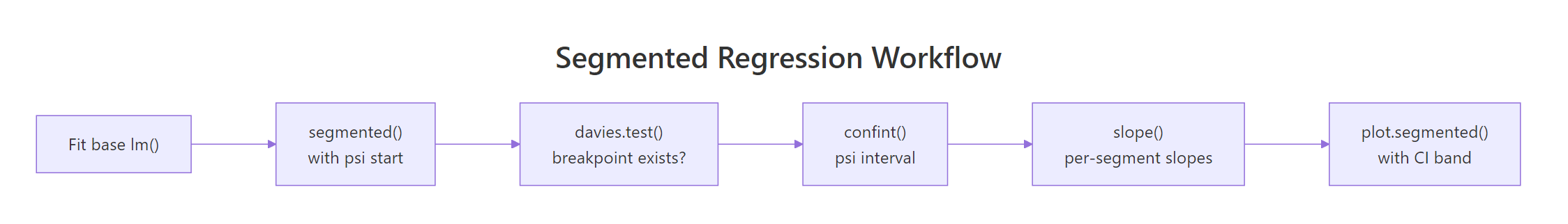
The segmented package workflow, from a base lm to a plotted fit with confidence intervals.

Figure 2: The segmented package workflow, from a base lm to a plotted fit with confidence intervals.

You already fit fit_seg in the first code block. Now print its full summary to read the four numbers that matter: intercept, pre-breakpoint slope, slope change at the kink (U1.x), and the breakpoint location.

RFull segmented summary

# Full summary of the segmented fit summary(fit_seg) #> ***Regression Model with Segmented Relationship(s)*** #> #> Estimated Break-Point(s): #> Est. St.Err #> psi1.x 29.85 0.481 #> #> Coefficients of the linear terms: #> Estimate Std. Error t value Pr(>|t|) #> (Intercept) -0.00876 0.39411 -0.022 0.982 #> x 0.21428 0.02211 9.690 < 2e-16 *** #> U1.x 0.76541 0.04357 17.568 ---

The row U1.x is the estimated slope change at the kink, the package's equivalent of our manual $\beta_2$. R flags its t-test with --- because the usual p-value is not valid when the breakpoint itself is estimated. For the slope change, use davies.test() instead (next section).

RPer-segment slopes with slope()

# slope() reports pre- and post-breakpoint slopes with SEs slope(fit_seg) #> $x #> Est. St.Err. t value CI(95%).l CI(95%).u #> slope1 0.2143 0.02211 9.6900 0.17091 0.2577 #> slope2 0.9797 0.03770 25.9900 0.90584 1.0535

Pre-breakpoint slope 0.21 and post-breakpoint slope 0.98 are the two numbers a reader wants: the dose-response is roughly flat below the threshold and rises steeply above it.

RConfidence interval for the breakpoint

# 95% CI for the breakpoint location confint(fit_seg) #> Est. CI(95%).l CI(95%).u #> psi1.x 29.85 28.90 30.80

The 95% interval [28.9, 30.8] contains the true value of 30. Report this interval whenever you report the breakpoint. A point estimate alone hides the uncertainty, which is often the most interesting number in a segmented analysis.

Tip

If you have no idea where the breakpoint is, pass psi = NA. segmented() will pick a quantile-based starting value automatically. This often works for simple cases but can fail on flat stretches, in which case an informed starting value from a scatter plot is safer.

Try it: Refit fit_lin with two different starting values, psi = 10 and psi = 50, and confirm both converge to roughly the same estimate. This is a quick sanity check that the estimate is not a local optimum.

RYour turn: refit with different starting values

# Fit with psi = 10 and psi = 50 ex_fit_10 <- # your code here ex_fit_50 <- # your code here # Print both breakpoint estimates c(from_10 = ex_fit_10$psi[, "Est."], from_50 = ex_fit_50$psi[, "Est."]) # Expected: both near 29.85

Click to reveal solution

RStarting-value sanity check solution

ex_fit_10 <- segmented(fit_lin, seg.Z = ~ x, psi = 10) ex_fit_50 <- segmented(fit_lin, seg.Z = ~ x, psi = 50) round(c(from_10 = ex_fit_10$psi[, "Est."], from_50 = ex_fit_50$psi[, "Est."]), 3) #> from_10 from_50 #> 29.852 29.852

Explanation: Both starting values converge to the same global optimum at 29.85, confirming the iterative algorithm found a stable breakpoint rather than a local minimum.

How do you test whether a breakpoint actually exists?

Here is the trap: segmented() always returns a breakpoint, even when the true relationship is a straight line. The algorithm will happily fit a kink to noise if you ask it to. You need a formal test for "does a breakpoint exist at all?" before trusting any of the estimates above.

davies.test() answers that question. It tests the null hypothesis that the slope is constant (no breakpoint) against the alternative that there is a breakpoint somewhere in the predictor's range. A small p-value rejects the null and supports the segmented fit.

Rdavies.test on threshold data

# davies.test on our kink data: expect a tiny p-value davies.test(fit_lin, seg.Z = ~ x) #> #> Davies' test for a change in the slope #> #> data: formula = y ~ x , method = lm #> model = gaussian , link = identity #> segmented variable = x #> 'best' at = 31.22, n.points = 10, p-value < 2.2e-16 #> alternative hypothesis: two.sided

p-value below 2.2e-16 is overwhelming evidence of a breakpoint. The "best at" value of 31.22 is the candidate breakpoint the test found most favourable; it is close to the segmented() estimate of 29.85 but uses a different grid, so slight differences are expected.

Rdavies.test on purely linear data

# Generate purely linear data and run the same test set.seed(99) x2 <- runif(120, 0, 60) y2 <- 0.4 * x2 + rnorm(120, sd = 1.5) fit_lin2 <- lm(y2 ~ x2) davies.test(fit_lin2, seg.Z = ~ x2) #> #> Davies' test for a change in the slope #> #> 'best' at = 28.30, n.points = 10, p-value = 0.6832

p-value 0.68 does not reject the null, so there is no evidence of a breakpoint. segmented() would still return a "breakpoint" if asked, but that number is fitted to noise and has no real meaning. Always davies.test first.

Warning

A significant davies.test does not validate the breakpoint location, only its existence. The test says "the slope changes somewhere." It does not say "the slope changes at the estimate you see." Always report confint(fit_seg) alongside the point estimate so readers see the uncertainty in location.

Try it: Run davies.test() on mpg ~ hp from mtcars. A small p-value would say horsepower's effect on mileage changes slope at some point. Interpret what you see.

RYour turn: davies.test on mtcars

# Fit base lm and run davies.test ex_mt_fit <- lm(mpg ~ hp, data = mtcars) # your code here # Is the p-value small or large? What does that say about mpg ~ hp?

Click to reveal solution

Rdavies.test on mtcars solution

ex_mt_fit <- lm(mpg ~ hp, data = mtcars) davies.test(ex_mt_fit, seg.Z = ~ hp) #> #> 'best' at = 97, n.points = 10, p-value = 0.002619

Explanation: The p-value of 0.0026 rejects the no-breakpoint null, so the mpg-hp relationship likely has a kink around 97 hp: cars below that lose mileage fast per extra horsepower, cars above that lose mileage more slowly. A segmented fit would quantify both slopes.

How do you fit multiple breakpoints?

Real data often has more than one regime change. segmented() handles multiple breakpoints in the same predictor by accepting a vector of starting values in psi. If you also don't know how many breakpoints there are, selgmented() picks the number for you using BIC or a sequence of davies tests.

Start by simulating three-segment data with kinks at x = 20 and x = 50, then fit the model with two starting breakpoints.

RSimulate and fit a three-segment model

# Three-segment data: slopes 0.2, 1.0, 0.3 with kinks at 20 and 50 set.seed(7) x3 <- runif(200, 0, 80) y3 <- 0.2 * x3 + ifelse(x3 > 20, 0.8 * (x3 - 20), 0) + ifelse(x3 > 50, -0.7 * (x3 - 50), 0) + rnorm(200, sd = 1.2) df3 <- data.frame(x = x3, y = y3) # Fit with two starting breakpoints fit_lin3 <- lm(y ~ x, data = df3) fit_seg3 <- segmented(fit_lin3, seg.Z = ~ x, psi = c(20, 50)) round(fit_seg3$psi[, c("Est.", "St.Err")], 3) #> Est. St.Err #> psi1.x 19.905 0.237 #> psi2.x 50.128 0.493

Both breakpoints recover within 0.2 of the true values. The standard errors pin down the first kink (0.24) tighter than the second (0.49), because the first regime has more data packed into it at the simulated range.

When you don't know the number of segments, use selgmented():

RChoose number of breakpoints with BIC

# selgmented picks K in [0, Kmax] via BIC fit_sel <- selgmented(fit_lin3, seg.Z = ~ x, Kmax = 3, type = "bic") fit_sel$selection.psi$npsi #> [1] 2

selgmented() returns 2, matching the true number of breakpoints. Under the hood, it fits models with 0, 1, 2, and 3 breakpoints, then picks the one with the best BIC.

Tip

BIC penalises extra breakpoints more strongly than AIC, so it resists overfitting to noise. For exploratory work where you want to be conservative about declaring kinks, BIC is usually the safer pick. For a stricter test, use type = "score" which performs sequential Davies tests at each candidate K.

Try it: Run selgmented() on df3 with type = "score" (sequential Davies tests). Does it select the same K = 2 as BIC?

RYour turn: compare BIC vs Davies selection

# Refit with sequential Davies testing ex_sel_score <- # your code here # Print selected K ex_sel_score$selection.psi$npsi # Expected: 2 (same as BIC)

Click to reveal solution

Rselgmented with score test solution

ex_sel_score <- selgmented(fit_lin3, seg.Z = ~ x, Kmax = 3, type = "score") ex_sel_score$selection.psi$npsi #> [1] 2

Explanation: Both BIC and sequential score tests agree on K = 2 breakpoints here because the signal is strong. In noisier data, the two criteria sometimes disagree, and BIC tends to be more conservative.

How do you plot segmented fits with confidence bands?

plot.segmented() draws the fitted broken line but not the raw data. Plot the points first, then overlay the fit. Pass conf.level = 0.95 to add a shaded pointwise confidence band.

RBase-R plot with confidence band

# Scatter first, then overlay the segmented fit with CI band plot(y ~ x, data = df_kink, pch = 20, col = "grey50", xlab = "x", ylab = "y") plot(fit_seg, add = TRUE, conf.level = 0.95, shade = TRUE, col = "steelblue", lwd = 2, rug = FALSE) # Vertical line at the breakpoint abline(v = fit_seg$psi[, "Est."], lty = 2, col = "firebrick")

The shaded band narrows away from the breakpoint and widens near it, because the model is least certain right where the slope flips. Readers who want one image of a segmented fit want this one: raw data, fitted break, visible uncertainty.

For a ggplot version, extract pointwise predictions and CI with broken.line():

Rggplot with pointwise confidence ribbon

# broken.line returns fitted values + SE on a fine grid br <- broken.line(fit_seg, se.fit = TRUE) plot_df <- data.frame( x = df_kink$x, fit = br$fit, lo = br$fit - 1.96 * br$se.fit, hi = br$fit + 1.96 * br$se.fit ) plot_df <- plot_df[order(plot_df$x), ] ggplot(df_kink, aes(x, y)) + geom_point(colour = "grey50", alpha = 0.6) + geom_ribbon(data = plot_df, aes(y = fit, ymin = lo, ymax = hi), fill = "steelblue", alpha = 0.3) + geom_line(data = plot_df, aes(y = fit), colour = "steelblue", linewidth = 1) + geom_vline(xintercept = fit_seg$psi[, "Est."], linetype = "dashed", colour = "firebrick") + theme_minimal()

Note

plot.segmented() draws the fit, not the raw data. If you skip the initial plot(y ~ x, ...) call, you get a broken line floating on a blank canvas. Always plot the scatter first, then overlay.

Try it: Recreate the ggplot above but colour the points by whether they sit before or after the estimated breakpoint, using the helper column df_kink$segment.

RYour turn: colour points by segment

# Add a segment column based on the fitted breakpoint psi_est <- fit_seg$psi[, "Est."] df_kink$segment <- ifelse(df_kink$x < psi_est, "pre", "post") # Now plot with colour = segment # your code here

Click to reveal solution

RSegment-coloured plot solution

psi_est <- fit_seg$psi[, "Est."] df_kink$segment <- ifelse(df_kink$x < psi_est, "pre", "post") ggplot(df_kink, aes(x, y, colour = segment)) + geom_point(alpha = 0.7) + geom_vline(xintercept = psi_est, linetype = "dashed") + scale_colour_manual(values = c(pre = "steelblue", post = "firebrick")) + theme_minimal()

Explanation: Splitting points by regime makes the two slopes visually distinct before you even add the fitted line, a quick way to convince a reader that the kink is real.

Practice Exercises

Exercise 1: Report the breakpoint with its 95% CI

Using df_kink from earlier in the tutorial, fit a segmented model, report the 95% confidence interval for the breakpoint, and confirm a davies test rejects the no-breakpoint null at the 1% level. Save the CI to my_psi_ci.

RExercise 1 starter: breakpoint with CI

# Fit lm and segmented, extract CI, run davies.test # Hint: segmented() then confint() then davies.test() # Write your code below:

Click to reveal solution

RExercise 1 solution

my_base <- lm(y ~ x, data = df_kink) my_seg <- segmented(my_base, seg.Z = ~ x, psi = 25) my_psi_ci <- confint(my_seg) my_psi_ci #> Est. CI(95%).l CI(95%).u #> psi1.x 29.85 28.90 30.80 davies.test(my_base, seg.Z = ~ x)$p.value #> [1] 2.220446e-16

Explanation: The CI [28.9, 30.8] and the Davies p-value below 1e-15 together say: yes, there is a breakpoint, and it is very likely between x = 28.9 and x = 30.8.

Exercise 2: Let selgmented choose K

Generate three-segment data with slopes 0.2, 1.0, 0.3 and breakpoints at 20 and 50, using set.seed(42) and 200 points. Fit a base lm() and use selgmented() with BIC to pick the number of breakpoints. Confirm it selects K = 2.

RExercise 2 starter: automatic K selection

# Generate data, fit base lm, then selgmented(..., Kmax=3, type='bic') # Write your code below:

Click to reveal solution

RExercise 2 solution

set.seed(42) my_x <- runif(200, 0, 80) my_y <- 0.2 * my_x + ifelse(my_x > 20, 0.8 * (my_x - 20), 0) + ifelse(my_x > 50, -0.7 * (my_x - 50), 0) + rnorm(200, sd = 1.2) my_df <- data.frame(x = my_x, y = my_y) my_base2 <- lm(y ~ x, data = my_df) my_sel <- selgmented(my_base2, seg.Z = ~ x, Kmax = 3, type = "bic") my_sel$selection.psi$npsi #> [1] 2

Explanation: BIC penalises extra breakpoints, so when the true K is 2, a K=3 model incurs a penalty without reducing the residual sum of squares enough to compensate. selgmented reports K=2.

Exercise 3: Segmented vs cubic spline by AIC

On df_kink, fit a cubic spline with splines::bs(x, df = 4) and compare its AIC to the segmented fit. Which model wins, and why should you not be surprised?

RExercise 3 starter: AIC comparison

# Fit the spline, then AIC(fit_seg, fit_spline) # Write your code below:

Click to reveal solution

RExercise 3 solution

library(splines) my_spline <- lm(y ~ bs(x, df = 4), data = df_kink) AIC(fit_seg, my_spline) #> df AIC #> fit_seg 5 444.2173 #> my_spline 6 451.7981

Explanation: The segmented fit wins by about 7 AIC units because the true data-generating process has a kink, and segmented regression spends its 5 parameters exactly where they are needed. The spline wastes degrees of freedom on smooth curvature that is not in the data.

Complete Example

Muggeo's stagnant dataset ships with the segmented package and is the textbook demonstration of a kink. It relates log-concentration of a chemical solution to a response; the slope changes sign around log.conc = -0.7.

RComplete segmented analysis on stagnant

# Load the canonical example data(stagnant) head(stagnant, 3) #> x y #> 1 -1.3862 1.005 #> 2 -1.2393 0.997 #> 3 -1.0876 0.988 # Fit base lm, then segmented with a psi guess from the scatter base_stag <- lm(y ~ x, data = stagnant) seg_stag <- segmented(base_stag, seg.Z = ~ x, psi = -0.7) # Breakpoint with 95% CI confint(seg_stag) #> Est. CI(95%).l CI(95%).u #> psi1.x -0.72 -0.74 -0.69 # Per-segment slopes slope(seg_stag)$x #> Est. St.Err. t value CI(95%).l CI(95%).u #> slope1 -0.4189 0.01360 -30.80 -0.4462 -0.3915 #> slope2 -1.0144 0.01245 -81.47 -1.0394 -0.9893 # Davies test to confirm the breakpoint is real davies.test(base_stag, seg.Z = ~ x)$p.value #> [1] 1.776357e-15 # Plot the fit plot(y ~ x, data = stagnant, pch = 20, col = "grey50", xlab = "log(concentration)", ylab = "response") plot(seg_stag, add = TRUE, conf.level = 0.95, shade = TRUE, col = "steelblue", lwd = 2, rug = FALSE) abline(v = seg_stag$psi[, "Est."], lty = 2, col = "firebrick")

The breakpoint sits at log.conc = -0.72 with a tight 95% CI of [-0.74, -0.69]. The slope switches from -0.42 before the breakpoint to -1.01 after, so the response falls roughly 2.4 times faster past the threshold. The Davies p-value of 1.8e-15 rules out "no kink" as an explanation.

Summary

Function	Purpose	When to use
`segmented()`	Estimate breakpoint + slopes	The main workhorse; always start here
`davies.test()`	Does a breakpoint exist at all	Before trusting any segmented fit
`confint()`	95% CI for breakpoint location	Always report alongside the point estimate
`slope()`	Per-segment slopes with SE	For interpretation of what changed
`selgmented()`	Choose number of breakpoints	When K is unknown; use BIC by default
`broken.line()`	Pointwise fitted + SE vectors	For ggplot ribbons or custom plots
`lm(y ~ x + pmax(x - c, 0))`	Manual fit with known breakpoint	Rare in practice; useful for teaching

Segmented regression shines when theory or a scatter plot shows an abrupt slope change at an unknown point. Pair segmented() with davies.test() so you never report a breakpoint that is not there, and always report a confidence interval so readers see the uncertainty in the location.

References

Muggeo, V. M. R. (2003). Estimating regression models with unknown break-points. Statistics in Medicine, 22(19), 3055-3071. Link
Muggeo, V. M. R. (2008). segmented: An R package to Fit Regression Models with Broken-Line Relationships. R News 8(1), 20-25. Link
Muggeo, V. M. R. (2016). Testing with a nuisance parameter present only under the alternative: a score-based approach with application to segmented modelling. Journal of Statistical Computation and Simulation, 86(15), 3059-3067. Link
Muggeo, V. M. R. (2017). Interval estimation for the breakpoint in segmented regression: a smoothed score-based approach. Australian & New Zealand Journal of Statistics, 59(3), 311-322. Link
Davies, R. B. (1987). Hypothesis testing when a nuisance parameter is present only under the alternative. Biometrika, 74(1), 33-43. Link
CRAN, segmented package reference manual. Link

Continue Learning

Polynomial and Spline Regression in R, when your scatter plot curves smoothly instead of kinking, reach for poly(), bs(), or mgcv::gam().
Regression Diagnostics in R, a systematic U-shape in the residuals-vs-fitted plot is the classic hint that a missing breakpoint is hiding inside your linear model.
Linear Regression Assumptions in R, segmented regression relaxes the constant-slope assumption; this post covers the other assumptions that still have to hold.

Segmented Regression in R: Breakpoints, Piecewise Linear & Threshold

When should you use segmented regression instead of polynomial or spline?

How do you fit segmented regression by hand with lm()?

How does segmented::segmented() estimate the breakpoint automatically?

How do you test whether a breakpoint actually exists?

How do you fit multiple breakpoints?

How do you plot segmented fits with confidence bands?

Practice Exercises

Exercise 1: Report the breakpoint with its 95% CI

Exercise 2: Let selgmented choose K

Exercise 3: Segmented vs cubic spline by AIC

Complete Example

Summary

References

Continue Learning

Related Tutorials

How do you fit segmented regression by hand with `lm()`?

How does `segmented::segmented()` estimate the breakpoint automatically?