Runs Test in R: Test Whether a Sequence Is Random
The Runs Test, also called the Wald-Wolfowitz Runs Test, checks whether a binary or dichotomized sequence was produced by a random process. It does this by counting consecutive same-value streaks (runs) and comparing that count against what randomness would predict.
What does the runs test actually measure?
Most randomness checks ask "is the distribution right?" The runs test asks something different: "is the order random?" A sequence can have the right balance of 1s and 0s yet still alternate too smoothly or clump too much. The fastest way to feel this is to push an obviously non-random sequence through tseries::runs.test() and watch what happens.
The Z statistic of -4.14 is more than four standard deviations below zero, and the p-value is 0.00003. With a clumped sequence we observed only 2 runs (one stretch of zeros, one stretch of ones), and that's far fewer than the 11 the test expected from a random sequence with this 10/10 split. The test correctly flags the order as non-random.
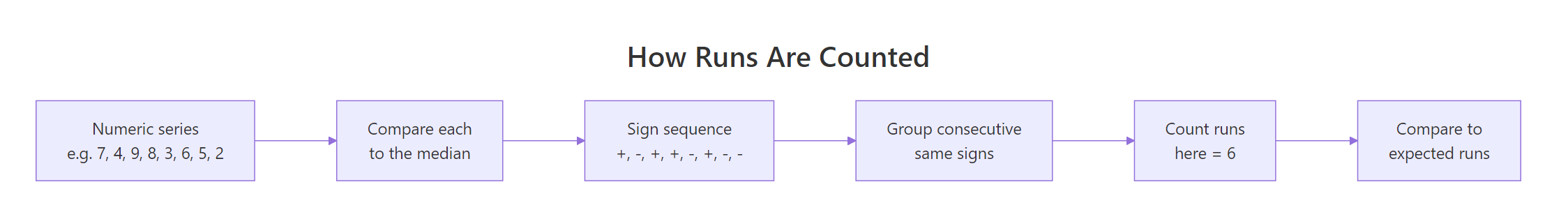
Figure 1: Dichotomizing a numeric series at its median, then counting runs of consecutive same-sign values.
Try it: Apply runs.test() to the perfectly clumped 8-element sequence below. Predict the sign of Z before running it.
Click to reveal solution
Explanation: Only 2 runs against an expected 5 → Z is negative (too few runs). The p-value barely clears 0.05 because n is small.
How do you run the runs test in R with tseries?
The tseries package's runs.test() requires a two-level factor as input. Passing a raw numeric vector silently coerces and can produce confusing results, so always wrap with factor() first. Once that's set up, the call is one line.
A p-value of 0.69 is well above 0.05, so we fail to reject the null hypothesis of randomness. The Z statistic is close to zero, meaning the observed run count is right where a random sequence would produce it.
The same call works on any two-level factor, it doesn't have to be 0/1. Coin tosses with "H" and "T" work just as well.
Again, no rejection. The test is symmetric in the two factor levels, relabelling 0/1 to H/T does not change the Z value.
runs.test() expects a 2-level factor and silently produces wrong results if you hand it a numeric vector with more than two unique values. Wrapping in factor() is cheap insurance.Try it: Sample 60 binary values with set.seed(7) and run the test. Report whether you reject H0.
Click to reveal solution
Explanation: p ≈ 0.43, far above 0.05, so we fail to reject randomness. The sequence shows no evidence of clumping or over-alternation.
How do you apply the runs test to continuous data?
The runs test only understands two categories. For a continuous variable like temperature or wind speed, dichotomize first by comparing each value to the median. Values above the median become "+" (or 1), values below become "−" (or 0). The median split keeps n1 and n2 close to equal, which gives the test the most power.
The p-value of 0.13 doesn't reach significance, but the negative Z hints at slight clumping, calmer days tend to follow calmer days, windier days follow windier days, which makes physical sense for daily weather.
The same dichotomization trick works for residuals from a fitted model. If a regression has captured all the structure in the data, the signs of its residuals should look like a random sequence.
The p-value here is far from significant. The residuals' signs alternate just enough, the linear model has absorbed the trend and what remains looks random.
The randtests package offers a runs.test() that accepts continuous input directly and dichotomizes by the median for you. The result is identical to the manual median-split approach shown above; pick whichever feels more readable.
Try it: Dichotomize airquality$Temp by its median and test for randomness.
Click to reveal solution
Explanation: Z ≈ -7.3 with a tiny p-value. Daily temperatures show strong serial dependence: warm days cluster together, so the sign sequence has far fewer runs than a random sequence would.
How do you interpret the Z statistic and p-value?
The runs test reduces to a Z-test on the count statistic R, the observed number of runs. With $n_1$ values above the split and $n_2$ values below, a random sequence has
$$\bar{R} \;=\; \frac{2\, n_1\, n_2}{n_1 + n_2} \;+\; 1$$
and variance
$$\operatorname{Var}(R) \;=\; \frac{2\, n_1\, n_2\, (2\, n_1\, n_2 - n_1 - n_2)}{(n_1 + n_2)^2 \, (n_1 + n_2 - 1)}.$$
The test statistic is then
$$Z \;=\; \frac{R - \bar{R}}{\sqrt{\operatorname{Var}(R)}},$$
and for moderate samples Z is approximately standard normal under the null.
Where:
- $R$ = the observed number of runs in your sequence
- $\bar{R}$ = the expected number of runs under randomness
- $\operatorname{Var}(R)$ = the variance of R under randomness
- $n_1, n_2$ = the counts of the two factor levels
That's all there is to it. Let's verify this against the tseries output by computing Z by hand on the 100-element random sequence from earlier.
The manual Z of 0.4045 and the manual p-value of 0.6859 match tseries exactly. The output of runs.test() is just this calculation wrapped in a print method.
The two-sided p-value rejects randomness in either direction: too few runs (clumping/trend) or too many runs (over-alternation, e.g., a regular high-low oscillation). To test only one direction, pass alternative = "less" (clumping) or alternative = "greater" (over-alternation) to runs.test().
Try it: With $n_1 = 15$, $n_2 = 15$, and $R = 10$ observed runs, compute Z by hand and the two-sided p-value.
Click to reveal solution
Explanation: Expected 16 runs, observed only 10 → Z ≈ −2.26 → p ≈ 0.024. We reject randomness at α = 0.05; the sequence is more clumped than chance.
When can the runs test mislead you?
The runs test has three failure modes worth knowing.
Small samples. The Z-approximation assumes $n \geq 20$ or so (some authors say $n_1, n_2 \geq 10$). Below that, the normal approximation is poor and you should rely on exact p-values when the package offers them. With very small n, even strong patterns may look insignificant.
A perfectly alternating sequence does reject here, but only just. For n = 6 it would not, the test simply doesn't have the resolution.
Periodicity that the test can't see. A sinusoidal pattern can produce roughly the expected number of runs while being highly structured. The runs test counts streak boundaries; it doesn't see periodicity. Pair it with an autocorrelation function (ACF) plot or a Ljung-Box test for time-series data.
Ties at the split point. When you dichotomize a continuous variable, values exactly equal to the median are ambiguous. Most implementations drop them or assign them to one side. With many ties, both choices change the answer materially.
Try it: Generate the sign sequence of sin(seq(0, 6 * pi, length.out = 30)) and run the test. Notice how it can miss obvious cyclic structure.
Click to reveal solution
Explanation: Even though the signs are blatantly periodic, the runs test only mildly suspects non-randomness (p ≈ 0.09). The number of runs is in the right ballpark, the test sees count, not pattern.
Practice Exercises
Exercise 1: Random walk sign sequence
Simulate a random walk of length 200 (cumulative sum of standard normal increments). Compute the sign of consecutive differences and run the test. Save the test object to my_walk_test.
Click to reveal solution
Explanation: The increments of a random walk are independent normals, so the sign sequence should be random. p ≈ 0.67 confirms it, the test has no evidence against randomness, exactly as theory predicts.
Exercise 2: Empirical Type-I error rate
Confirm that under H0 the runs test rejects roughly 5% of the time at α = 0.05. Generate 1000 random binary sequences of length 50, run the test on each, and compute the rejection rate. Save it to my_reject_rate.
Click to reveal solution
Explanation: About 5.4% of the 1000 simulated random sequences are rejected at α = 0.05, very close to the nominal 5%. The test's Type-I error rate matches its design.
Complete Example: checking regression residuals for randomness
Linear regression assumes the residuals are uncorrelated. After fitting a model on time-ordered data, the signs of the residuals should form a random sequence. If they don't, the model is missing structure, typically a nonlinear term or an autocorrelation pattern.
We'll fit Ozone ~ Temp on the airquality dataset, check the residual signs, and interpret the result.
The p-value of 0.01 rejects randomness. The residuals' signs are clumped, long runs of positive then long runs of negative residuals, which is a textbook sign that a linear-only Temp term has missed curvature in the relationship. A quadratic term or a more flexible model would likely fix it.
This single test is fast, assumption-light, and gives a clear pass/fail signal. It is a good first-line check before you reach for more elaborate diagnostics.
Summary
| Question the test answers | Is the order of a 2-level sequence random? |
|---|---|
| Required input | A factor with exactly 2 levels (or a continuous vector you dichotomize) |
| R function | tseries::runs.test() |
| Test statistic | Z = (R − E[R]) / sqrt(Var[R]) |
| Decision rule | Reject H0 of randomness when p < 0.05 |
| Common pitfalls | Small n, ties at the median, periodicity invisible to runs |
| Best paired with | An ACF plot or a Ljung-Box test for time-series checks |
One-line recipe for any continuous series x:
References
- Wald, A. & Wolfowitz, J. (1940). On a test whether two samples are from the same population. Annals of Mathematical Statistics, 11(2), 147-162. Link
- NIST/SEMATECH e-Handbook of Statistical Methods, 1.3.5.13. Runs Test for Detecting Non-randomness. Link
- tseries package documentation,
runs.test(). Link - randtests package, Testing Randomness in R. Link
- Bradley, J. V. (1968). Distribution-Free Statistical Tests. Prentice Hall.
- R Core Team, An Introduction to R. Link
Continue Learning
- When to Use Nonparametric Tests in R, the parent decision guide that places the runs test in the broader nonparametric toolbox.
- Autocorrelation in Residuals, the natural follow-up when a runs test on residual signs flags non-randomness.
- Mann-Whitney U Test in R, another rank-based, distribution-free test for two-sample comparisons.