tidyr expand() & complete() in R: Make Implicit Missing Values Explicit

Sometimes your data hides rows that should be there but aren't, a month with zero sales, a panel subject who skipped a visit, a date with no trades. These are implicit missing values, and they break plots, models, and joins silently. tidyr's expand() and complete() drag those gaps into the open as explicit NAs you can then fill.

Why should you care about implicit missing values?

Picture a small sales table: three products, three months, but only five rows because some products didn't sell in some months. Nothing looks wrong until you plot monthly totals and a whole column is missing. Rows that should exist but don't are called implicit missing values. complete() turns them into real rows you can see and handle, here's the one-liner that does it.

Five rows went in, nine rows came out. The four new rows carry NA in the units column, those are the combinations that were missing entirely from the raw data. You can now spot them, fill them, or count them. Before complete() they were invisible.

How does expand() build all combinations?

Before fixing implicit misses, it helps to see them. expand() is the inspection tool: given a data frame and a set of columns, it returns every unique combination of those columns, and only those columns. The row count of the result has nothing to do with the row count of the input.

Notice the units column is gone, expand() returns the grid alone, not your data joined to it. Use this when you want a clean scaffold you can compare against the original. Think of it as the "what should exist" blueprint.

If you want to build a grid from bare vectors, without any data frame involved, reach for crossing(). It's expand()'s standalone sibling and accepts named arguments directly.

Same nine rows, but crossing() never touches the sales tibble. This matters when you want the full expected universe of values regardless of what the data contains, for example, every month in a fiscal year whether or not sales were logged.

How does complete() fill missing combinations?

complete() is expand() plus dplyr::full_join() plus tidyr::replace_na() rolled into one call. You give it the columns to expand and it returns your original data with missing combinations inserted and optional default values filled in.

The fill argument takes a named list. Each name is a column; each value is what NAs in that column should become for the newly created rows.

Same nine rows as before, but now the previously-NA units are zero, the right default when "no sale" means "zero units sold." You can pass several columns at once: fill = list(units = 0, revenue = 0, discount = 0).

What if the raw data already contains a real NA that you want to preserve, say, a genuinely unknown sale? By default complete() replaces it along with the new NAs. Set explicit = FALSE (tidyr 1.2+) and the fill list only touches the rows complete() just added.

Jan/B keeps its original NA because the row already existed in the data. Only Feb/B, a brand-new row, gets the default zero. This distinction matters when "we don't know" and "definitely zero" mean different things in your analysis.

How do you fill missing dates in a time series?

The most common real-world use of complete() is filling date gaps. Your data might log daily sales, website visits, or sensor readings, but on days with no activity, no row gets written. complete() plus seq.Date() rebuilds the full calendar.

Pass the date sequence as a named argument to complete(). The name is the column; the value is the full range of values you want to see.

The two missing days (March 3 and March 6) now appear as proper rows with NA visit counts. A downstream plot will draw gaps where there were gaps; a forecasting model can now see that the time series is regular.

A common next step is to carry the last observation forward. tidyr::fill() handles that, the .direction = "down" argument says "copy the previous non-NA value downward."

March 3 inherits March 2's count; March 6 inherits March 5's. That's last-observation-carried-forward, the workhorse of time-series imputation when "no data" really means "no change reported."

When should you use nesting() instead?

Sometimes two columns describe the same entity, a patient_id and their diagnosis, a product_code and its category, an employee and their department. These columns are linked, not independent, so you never want to mix one patient with another patient's diagnosis. That's exactly what raw complete() would do.

nesting() tells tidyr: "treat these columns as a unit, only the combinations that already appear together in the data are valid."

Raw complete() produced 12 nonsense rows that paired every patient with every diagnosis, including diagnoses they never had. complete(nesting(patient_id, diagnosis), visit) keeps each (patient_id, diagnosis) pair exactly as it appeared and crosses it with every visit. The only new row is patient 3's V2, which is genuinely missing.

How do expand() and complete() work with groups?

When you apply complete() to a group_by()-ed tibble, it completes each group independently. That's exactly what you want for multi-site panels: every clinic, store, or region gets its own complete grid without cross-pollination.

North has all four product × month pairs, and so does South, each region independently. The grouping column region isn't expanded (you can't complete() a grouping column; tidyr will error if you try), which is the safe default.

Practice Exercises

Two capstone problems that combine several tools from this tutorial. The variable names start with my_ so they don't collide with the tutorial's tibbles.

Exercise 1: Fill a stock price panel

You have daily close prices for two tickers across five business days, but a few rows are missing. Produce a filled panel where every ticker has every date and any missing closes are carried forward from the previous day.

Exercise 2: Find missing student-exam pairs without adding rows

Given a grades tibble that's incomplete, return a data frame listing only the (student, exam) pairs where no grade exists, without touching the original.

Complete Example

Here is an end-to-end pipeline that ties everything together. The raw regional_sales_raw tibble has gaps across regions, products, and months. The goal is per-region monthly totals, and those totals will be wrong unless every region has a row for every product in every month.

Without the complete() step, North's March total would count only product B (six units) and omit product A entirely, even though the "correct" interpretation is that A sold zero units. After completion, the totals are consistent across regions, months, and products, and a downstream plot will show all three months for both regions without gaps in the x-axis.

Summary

Key takeaways:

• Tidy data has a row for every combination that should exist, even if the measurement is NA.
• complete() equals expand() plus dplyr::full_join() plus tidyr::replace_na() in a single call.
• Use nesting() for columns that describe the same entity; pass raw arguments for genuinely independent columns.
• Pass sequences by name for dates (seq.Date) and numerics (full_seq) to expand to a known universe.
• group_by() |> complete() gives each group its own independent grid, ideal for multi-site panels.

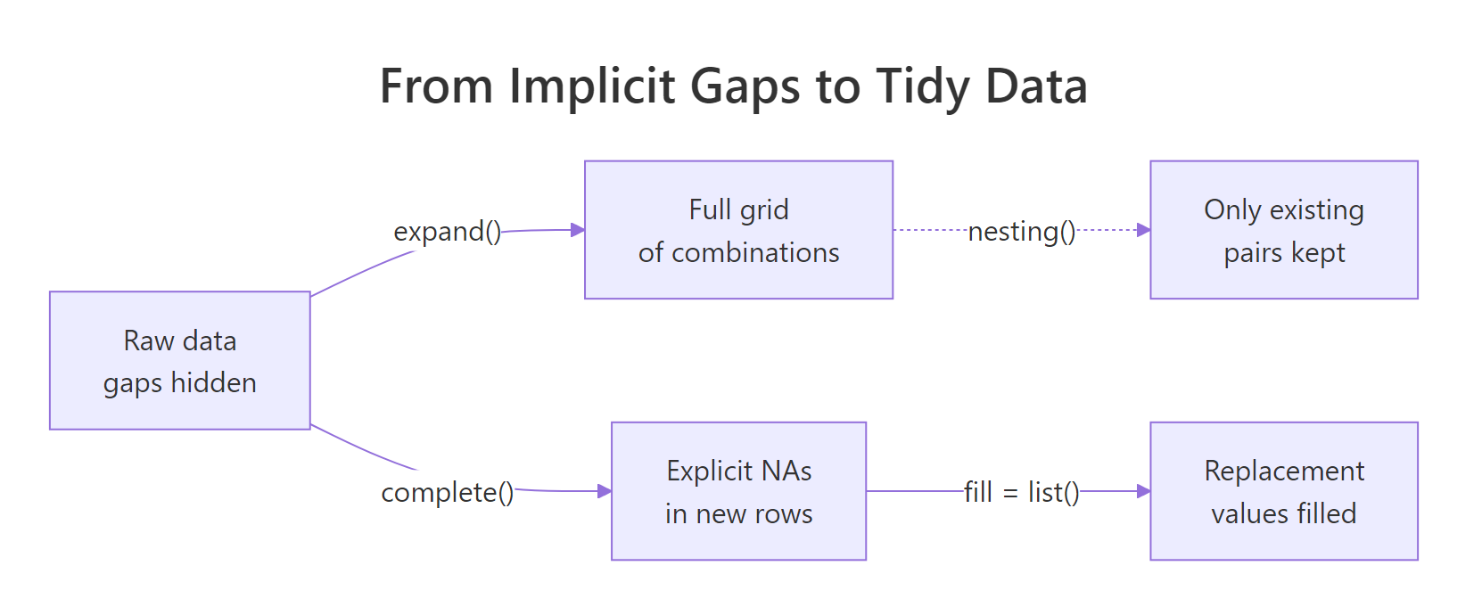
Figure 1: From raw data with gaps, expand() builds the full grid, complete() fills in explicit NAs, and a fill list replaces them with sensible defaults.

References

1. tidyr documentation, complete(). Link
2. tidyr documentation, expand() and crossing(). Link
3. tidyr documentation, full_seq(). Link
4. Wickham, H. & Grolemund, G., R for Data Science (2e), Chapter 18: Missing values. Link
5. tidyr 1.2.0 release notes, introduces the explicit argument. Link
6. tidyr documentation, fill() for carry-forward imputation. Link

Continue Learning

• pivot_longer() and pivot_wider(): Reshape Data in R Without Losing Your Mind, the parent reshaping guide that sets up why long data so often needs completing.
• Missing Values in R: Detect, Count, Remove, and Impute NA, once gaps are explicit NAs, learn how to count, visualise, and impute them.
• tidyr separate() & unite() in R: Split & Combine Character Columns, the sibling tidyr helper pair for splitting and rejoining character columns.