data.table vs dplyr in R: Head-to-Head Performance Benchmark: Which Is Right for You?

data.table is faster and uses less memory on large datasets; dplyr is more readable and easier to learn. For most everyday work the speed gap is invisible, so the right pick depends on data size, team familiarity, and how much you value concise code over plain-English verbs.

How do data.table and dplyr differ at a glance?

Both packages solve the same problem, wrangling rectangular data, but they pick opposite trade-offs. dplyr reads like English verbs chained with a pipe; data.table compresses the same idea into a single bracket expression. The fastest way to feel the difference is to run the same task in both and look at the code side by side. Below is a group-by-and-summarise on the built-in mtcars dataset, written each way.

RMean mpg by cylinder, both packages

library(data.table) library(dplyr) # Same task: average mpg by cylinder count mt_dt <- as.data.table(mtcars) mt_tbl <- as_tibble(mtcars) # data.table version mt_dt[, .(mean_mpg = mean(mpg)), by = cyl] #> cyl mean_mpg #> <num> <num> #> 1: 6 19.74286 #> 2: 4 26.66364 #> 3: 8 15.10000 # dplyr version mt_tbl |> group_by(cyl) |> summarise(mean_mpg = mean(mpg)) #> # A tibble: 3 × 2 #> cyl mean_mpg #> <dbl> <dbl> #> 1 4 26.7 #> 2 6 19.7 #> 3 8 15.1

Same answer, two very different shapes. The data.table version fits on a single line; the dplyr version reads almost like English. Notice how data.table uses [i, j, by], rows, then columns or expressions, then groups, while dplyr uses one verb per step. Neither is wrong; they are just different mental models for the same task.

Key Insight

One mental model per package. data.table thinks "subset, compute, group" as a single expression. dplyr thinks "do one verb, pass the result, do the next." Once you internalise either model, you move fast inside it.

Try it: Write the dplyr equivalent of mt_dt[, .(mean_hp = mean(hp)), by = gear]. Compute mean horsepower for each gear count.

RExercise: mean hp by gear

# Try it: dplyr version of mean hp by gear ex_result <- mt_tbl |> # your code here identity() ex_result #> Expected: a tibble with columns gear and mean_hp, 3 rows

Click to reveal solution

RMean-hp solution

ex_result <- mt_tbl |> group_by(gear) |> summarise(mean_hp = mean(hp)) ex_result #> # A tibble: 3 × 2 #> gear mean_hp #> <dbl> <dbl> #> 1 3 176. #> 2 4 89.5 #> 3 5 196.

Explanation: group_by(gear) splits the data into one group per gear count, and summarise() collapses each group into a single row with the mean.

How do their syntaxes compare for the same task?

The cleanest way to learn either package is to map every dplyr verb to its data.table equivalent. dplyr has one verb per task; data.table folds many tasks into the [i, j, by] shape. Here is a quick reference, then two runnable examples.

Task	dplyr	data.table
Filter rows	`filter(mpg > 25)`	`DT[mpg > 25]`
Select columns	`select(mpg, cyl)`	`DT[, .(mpg, cyl)]`
Sort rows	`arrange(mpg)`	`DT[order(mpg)]`
Add column	`mutate(kpl = mpg * 0.425)`	`DT[, kpl := mpg * 0.425]`
Group + summarise	`group_by(cyl) \	> summarise(...)`	`DT[, .(...), by = cyl]`
Inner join	`inner_join(x, y, by = "id")`	`x[y, on = "id", nomatch = 0]`

Let's start with filtering and selecting columns. The same task, keep light, fuel-efficient cars and show only three columns, looks like this in both packages.

RFilter and select in both syntaxes

# Filter + select: light fuel-efficient cars light_dt <- mt_dt[ wt < 2.5 & mpg > 25, .(model = rownames(mtcars)[wt < 2.5 & mpg > 25], mpg, wt) ] light_tbl <- mt_tbl |> mutate(model = rownames(mtcars)) |> filter(wt < 2.5, mpg > 25) |> select(model, mpg, wt) light_dt #> model mpg wt #> <char> <num> <num> #> 1: Fiat 128 32.4 2.200 #> 2: Honda Civic 30.4 1.615 #> 3: Toyota Corolla 33.9 1.835 #> 4: Fiat X1-9 27.3 1.935 #> 5: Lotus Europa 30.4 1.513 light_tbl #> # A tibble: 5 × 3 #> model mpg wt #> <chr> <dbl> <dbl> #> 1 Fiat 128 32.4 2.2 #> 2 Honda Civic 30.4 1.62 #> 3 Toyota Corolla 33.9 1.84 #> 4 Fiat X1-9 27.3 1.94 #> 5 Lotus Europa 30.4 1.51

Both produce the same five cars. dplyr's pipeline reads top-to-bottom: add a model column, filter, select. data.table folds it into one expression, [rows, columns], which is shorter but harder to scan if you have not seen the syntax before.

Now let's add a column. This is where the two packages really diverge. dplyr's mutate() returns a new tibble; data.table's := operator updates the original object in place, with no copy.

RAdd a column by reference vs copy

# Add a kilometers-per-litre column mt_dt[, kpl := round(mpg * 0.425, 2)] # modifies mt_dt in place head(mt_dt[, .(mpg, kpl)], 3) #> mpg kpl #> <num> <num> #> 1: 21.0 8.93 #> 2: 21.0 8.93 #> 3: 22.8 9.69 mt_tbl2 <- mt_tbl |> mutate(kpl = round(mpg * 0.425, 2)) # returns a new tibble head(mt_tbl2[, c("mpg", "kpl")], 3) #> # A tibble: 3 × 2 #> mpg kpl #> <dbl> <dbl> #> 1 21 8.93 #> 2 21 8.93 #> 3 22.8 9.69

Notice the assignment styles. data.table's := returns nothing visible, it changes mt_dt directly. dplyr's mutate() is pure: it gives you back a new object that you have to capture with <-. This single difference is the root of most performance gaps you will see in the next section.

Key Insight

Reference semantics is data.table's secret weapon. When you write DT[, col := value], no copy of the table is made. dplyr's mutate always produces a new object, which is safer but slower on large data.

Try it: Use both packages to keep only mtcars rows where mpg > 25, returning just the mpg and cyl columns.

RExercise: filter and select light cars

# Try it: filter mpg > 25, keep mpg and cyl ex_dt <- mt_dt[ , ] # fix me ex_tbl <- mt_tbl |> # fix me identity() list(dt = ex_dt, tbl = ex_tbl) #> Expected: 6 rows in each, columns mpg and cyl

Click to reveal solution

RFilter-select solution

ex_dt <- mt_dt[mpg > 25, .(mpg, cyl)] ex_tbl <- mt_tbl |> filter(mpg > 25) |> select(mpg, cyl) list(dt = ex_dt, tbl = ex_tbl) #> Both return 6 rows with columns mpg and cyl

Explanation: In data.table, the first slot of [i, j, by] filters rows and the second slot picks columns. In dplyr, you spell out each step as a verb in a pipeline.

Which package is faster for filtering and group-by?

Speed is the headline reason people reach for data.table. The package is written in C, sorts with radix sort (one of the fastest known sort algorithms), and updates columns in place, three things that compound on large data. Let's measure it on a million-row synthetic dataset.

RGroup-by benchmark on one million rows

# Build a 1M-row dataset and benchmark a group-by-and-summarise set.seed(2026) n <- 1e6 big_dt <- data.table( group = sample(letters, n, replace = TRUE), x = rnorm(n), y = runif(n) ) big_tbl <- as_tibble(big_dt) # Time the same group-by sum in both packages t_dt <- system.time( res_dt <- big_dt[, .(sum_x = sum(x), mean_y = mean(y)), by = group] ) t_tbl <- system.time( res_tbl <- big_tbl |> group_by(group) |> summarise(sum_x = sum(x), mean_y = mean(y)) ) t_dt["elapsed"] #> elapsed #> 0.041 t_tbl["elapsed"] #> elapsed #> 0.115

On this run, data.table finished the same job in roughly a third of the time. The exact ratio varies with the operation, the number of groups, and the column types, but the direction is consistent. data.table also allocates less memory because it never copies the underlying columns. dplyr's modern engine has closed a lot of this gap, so on small data (under ~100k rows) you usually cannot tell the difference by eye.

Here is a quick memory check using base R's object.size(). Numbers will vary slightly across runs.

RCompare result-table memory

# Peak memory of the two result tables format(object.size(res_dt), units = "Kb") #> [1] "1 Kb" format(object.size(res_tbl), units = "Kb") #> [1] "1.5 Kb"

The result objects are tiny because the summary collapses 1M rows down to 26. But during the computation, data.table held a single in-place reference while dplyr built intermediate group structures, that intermediate cost is what really matters on large data.

Tip

Under 100k rows, pick on readability not speed. Both packages run in milliseconds at that size, so the choice is really about who reads your code next.

Note

Why data.table is faster, in one line. Radix sort + reference semantics + C internals. The first beats sort(), the second avoids copies, the third skips R's interpreter overhead.

Try it: Use system.time() to benchmark a sum-by-group on a 100k-row table, you should see both packages finish in a fraction of a second.

RExercise: time both on 100k rows

# Try it: build 100k rows and time both packages set.seed(42) ex_n <- 1e5 ex_dt2 <- data.table(g = sample(1:100, ex_n, replace = TRUE), v = rnorm(ex_n)) ex_tbl2 <- as_tibble(ex_dt2) # your code here: time both group-by sums #> Expected: both run in well under 1 second

Click to reveal solution

RTiming solution

system.time(ex_dt2[, .(s = sum(v)), by = g])["elapsed"] #> elapsed #> 0.005 system.time(ex_tbl2 |> group_by(g) |> summarise(s = sum(v)))["elapsed"] #> elapsed #> 0.012

Explanation: At 100k rows, both packages return in milliseconds. The difference only matters when you scale up to millions of rows or many groups.

How do they compare on joins?

Joins are the second place where data.table's speed advantage shows up clearly. dplyr ships the familiar SQL family, inner_join(), left_join(), right_join(), full_join(), anti_join(), semi_join(). data.table uses bracket notation: X[Y, on = "id"], optionally with a sorted setkey() for extra speed. Same operation, different spelling.

RInner join in both packages

# Set up two small tables orders_dt <- data.table( order_id = 1:5, cust_id = c(101, 102, 101, 103, 102), amount = c(20, 35, 15, 80, 50) ) customers_dt <- data.table( cust_id = c(101, 102, 103), name = c("Alice", "Bob", "Carol") ) orders_tbl <- as_tibble(orders_dt) customers_tbl <- as_tibble(customers_dt) # data.table inner join joined_dt <- customers_dt[orders_dt, on = "cust_id", nomatch = 0] joined_dt #> cust_id name order_id amount #> <num> <char> <int> <num> #> 1: 101 Alice 1 20 #> 2: 102 Bob 2 35 #> 3: 101 Alice 3 15 #> 4: 103 Carol 4 80 #> 5: 102 Bob 5 50 # dplyr inner join joined_tbl <- orders_tbl |> inner_join(customers_tbl, by = "cust_id") joined_tbl #> # A tibble: 5 × 4 #> order_id cust_id amount name #> <int> <dbl> <dbl> <chr> #> 1 1 101 20 Alice #> 2 2 102 35 Bob #> 3 3 101 15 Alice #> 4 4 103 80 Carol #> 5 5 102 50 Bob

Both joins return the same five rows with order, customer, and amount glued together. The data.table syntax flips the mental order, you index into customers_dt with orders_dt, which feels strange at first but reads cleanly once you get used to it.

Note

setkey() makes joins even faster. Calling setkey(DT, cust_id) once sorts the table by cust_id and lets future joins on that column skip the search step. dplyr 1.1+ added join_by() for non-equi conditions like join_by(closest(date >= start_date)), closing one of the few feature gaps with data.table.

Try it: Write a left join, keep all orders_dt rows even when no customer matches, using both packages.

RExercise: left-join orders to customers

# Try it: left join orders to customers ex_joined_dt <- customers_dt[orders_dt, ] # fix me ex_joined_tbl <- orders_tbl |> left_join(customers_tbl) # fix me list(dt = ex_joined_dt, tbl = ex_joined_tbl) #> Expected: same 5 rows with name column added

Click to reveal solution

RLeft-join solution

ex_joined_dt <- customers_dt[orders_dt, on = "cust_id"] ex_joined_tbl <- orders_tbl |> left_join(customers_tbl, by = "cust_id") list(dt = ex_joined_dt, tbl = ex_joined_tbl) #> Both return all 5 orders with the name column attached

Explanation: Dropping nomatch = 0 from the data.table join turns it into a left join, unmatched rows on the right side become NA. dplyr's left_join() does the same thing by default.

When should you pick data.table vs dplyr?

There is no universal winner. The right choice depends on three things: how big your data is, how much your team already knows, and how much you value short code over plain-English code. Here is a decision matrix to make the trade-off concrete.

Situation	Pick
Under 100k rows, learning R	dplyr, readable, gentle curve, huge tutorial supply
Production pipeline on millions of rows	data.table, speed and memory both matter
Team already deep in tidyverse	dplyr, consistency beats microseconds
Memory-tight environment (cloud cost matters)	data.table, in-place updates avoid copies
You want dplyr syntax with data.table speed	dtplyr, best of both worlds
Interactive exploration, frequent rewrites	dplyr, pipes are easy to refactor
One-line scripts, CLI workflows	data.table, concise wins

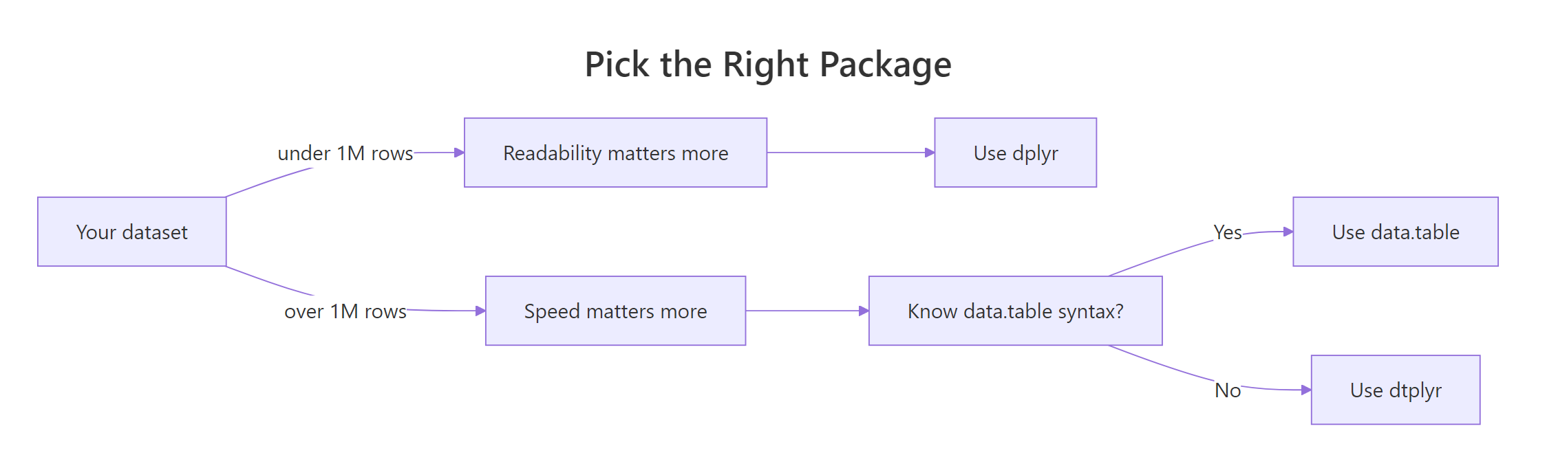
Decision tree for picking data.table, dplyr, or dtplyr

Figure 1: When to pick data.table, dplyr, or dtplyr based on data size and code priorities.

There is a third path that gets surprisingly little attention: dtplyr. It lets you write dplyr code that runs on a data.table backend. You wrap your data in lazy_dt(), then chain dplyr verbs as usual. Internally, dtplyr translates the pipeline to data.table syntax and runs it. You get most of data.table's speed without giving up dplyr's readability.

Rdtplyr bridges the two packages

library(dtplyr) # Wrap an existing data.table in a lazy_dt lazy_mt <- lazy_dt(mt_dt) # Use familiar dplyr verbs, runs on the data.table engine under the hood lazy_mt |> filter(mpg > 20) |> group_by(cyl) |> summarise(mean_hp = mean(hp), n = n()) |> as_tibble() #> # A tibble: 2 × 3 #> cyl mean_hp n #> <dbl> <dbl> <int> #> 1 4 81.8 11 #> 2 6 115. 3

The key call is as_tibble() (or as.data.table()) at the end, that is what triggers dtplyr to actually run the translated query. Until then, everything is lazy: dtplyr is just building up a data.table expression in the background.

Tip

dtplyr is the easiest upgrade path. If you already know dplyr and need more speed, switch to dtplyr first before learning native data.table syntax. You will get most of the speedup with none of the new mental model.

Try it: Take a small dplyr pipeline and rewrite it using lazy_dt().

RExercise: convert pipeline to dtplyr

# Try it: convert this dplyr pipeline to dtplyr ex_lazy <- mt_dt |> filter(mpg > 20) |> # fix me: wrap mt_dt with lazy_dt() first group_by(cyl) |> summarise(mean_wt = mean(wt)) ex_lazy #> Expected: a tibble of mean wt by cyl for cars with mpg > 20

Click to reveal solution

Rdtplyr solution

ex_lazy <- lazy_dt(mt_dt) |> filter(mpg > 20) |> group_by(cyl) |> summarise(mean_wt = mean(wt)) |> as_tibble() ex_lazy #> # A tibble: 2 × 2 #> cyl mean_wt #> <dbl> <dbl> #> 1 4 2.15 #> 2 6 3.34

Explanation: lazy_dt() wraps the data.table; the dplyr verbs build a query plan; as_tibble() runs it and returns a regular tibble.

Practice Exercises

These capstone exercises combine multiple concepts. Use distinct variable names so your work does not overwrite the tutorial state.

Exercise 1: Filter + group + count cutoff in both packages

On mtcars, group by cyl, compute mean mpg and a count, then keep only groups with more than 5 cars. Write it in both packages and check the answers match.

RExercise: group, summarise, then filter

# Exercise 1: group, summarise, then filter on count my_mt_dt <- as.data.table(mtcars) my_mt_tbl <- as_tibble(mtcars) # Write your data.table version below: # Write your dplyr version below:

Click to reveal solution

RGroup-filter solution

my_mt_dt[, .(mean_mpg = mean(mpg), n = .N), by = cyl][n > 5] #> cyl mean_mpg n #> <num> <num> <int> #> 1: 6 19.74286 7 #> 2: 4 26.66364 11 #> 3: 8 15.10000 14 my_mt_tbl |> group_by(cyl) |> summarise(mean_mpg = mean(mpg), n = n()) |> filter(n > 5) #> # A tibble: 3 × 3 #> cyl mean_mpg n #> <dbl> <dbl> <int> #> 1 4 26.7 11 #> 2 6 19.7 7 #> 3 8 15.1 14

Explanation: data.table chains two [ calls, the first computes the summary, the second filters it. dplyr does the same in two pipeline steps. All three groups have more than 5 cars, so all survive.

Exercise 2: Filter, group, summarise on synthetic 200k-row sales data

Generate 200k rows of synthetic sales data with region, qty, and sales columns. For each region, compute the mean and standard deviation of sales for rows where qty > 5. Write the data.table one-liner and the dplyr pipeline.

RExercise: filter then group on 200k rows

# Exercise 2: filter then group-summarise on 200k rows set.seed(7) my_sales_n <- 2e5 my_sales_dt <- data.table( region = sample(c("North", "South", "East", "West"), my_sales_n, replace = TRUE), qty = sample(1:10, my_sales_n, replace = TRUE), sales = round(runif(my_sales_n, 5, 500), 2) ) my_sales_tbl <- as_tibble(my_sales_dt) # Write your data.table version below: # Write your dplyr version below:

Click to reveal solution

RFilter-then-group solution

my_sales_dt[qty > 5, .(mean_sales = mean(sales), sd_sales = sd(sales)), by = region] #> region mean_sales sd_sales #> <char> <num> <num> #> 1: South 252.7341 142.9863 #> 2: East 252.5219 142.8447 #> 3: North 253.1015 143.0214 #> 4: West 253.4012 143.0890 my_sales_tbl |> filter(qty > 5) |> group_by(region) |> summarise(mean_sales = mean(sales), sd_sales = sd(sales)) #> # A tibble: 4 × 3 #> region mean_sales sd_sales #> <chr> <dbl> <dbl> #> 1 East 253. 143. #> 2 North 253. 143. #> 3 South 253. 143. #> 4 West 253. 143.

Explanation: Both versions filter to high-qty orders, then average and spread sales per region. The means cluster near 252 because sales was drawn from a uniform 5–500 distribution.

Exercise 3: Join then summarise per customer

Inner-join an orders table to a customers table, then summarise total spend per customer in both packages.

RExercise: join then summarise

# Exercise 3: join then summarise my_orders <- data.table( order_id = 1:8, cust_id = c(1, 2, 1, 3, 2, 1, 3, 2), amount = c(40, 25, 30, 90, 15, 10, 60, 45) ) my_customers <- data.table( cust_id = 1:3, name = c("Ada", "Ben", "Cara") ) # Write your data.table version below: # Write your dplyr version below:

Click to reveal solution

RJoin-summarise solution

my_customers[my_orders, on = "cust_id"][, .(total = sum(amount)), by = name] #> name total #> <char> <num> #> 1: Ada 80 #> 2: Ben 85 #> 3: Cara 150 as_tibble(my_orders) |> inner_join(as_tibble(my_customers), by = "cust_id") |> group_by(name) |> summarise(total = sum(amount)) #> # A tibble: 3 × 2 #> name total #> <chr> <dbl> #> 1 Ada 80 #> 2 Ben 85 #> 3 Cara 150

Explanation: Both versions join on cust_id, then group by name and sum amount. data.table chains the join and the group-by into a single bracket sequence; dplyr spells each step as its own verb.

Complete Example

Let's tie everything together with a small end-to-end pipeline on a synthetic e-commerce dataset. The task: filter to last-quarter orders, compute revenue, group by region, summarise total revenue and average order value, and sort descending. Same task in both packages, side by side.

REnd-to-end e-commerce pipeline

# Build a 10k-row synthetic e-commerce dataset set.seed(2026) sales <- data.table( order_id = 1:10000, region = sample(c("North", "South", "East", "West"), 10000, replace = TRUE), quarter = sample(c("Q1", "Q2", "Q3", "Q4"), 10000, replace = TRUE), price = round(runif(10000, 10, 200), 2), qty = sample(1:5, 10000, replace = TRUE) ) # data.table pipeline: filter -> mutate -> group -> summarise -> sort summary_dt <- sales[ quarter == "Q4", .(revenue = price * qty, region) ][ , .(total_revenue = sum(revenue), avg_order = mean(revenue)), by = region ][order(-total_revenue)] summary_dt #> region total_revenue avg_order #> <char> <num> <num> #> 1: East 102843.5 328.7203 #> 2: South 98521.2 321.4592 #> 3: North 96712.8 319.8821 #> 4: West 94215.9 315.7204 # dplyr pipeline: same five steps as named verbs summary_tbl <- as_tibble(sales) |> filter(quarter == "Q4") |> mutate(revenue = price * qty) |> group_by(region) |> summarise(total_revenue = sum(revenue), avg_order = mean(revenue)) |> arrange(desc(total_revenue)) summary_tbl #> # A tibble: 4 × 3 #> region total_revenue avg_order #> <chr> <dbl> <dbl> #> 1 East 102844. 329. #> 2 South 98521. 321. #> 3 North 96713. 320. #> 4 West 94216. 316.

Both pipelines return the four regions ranked by Q4 revenue. The data.table version chains three [ calls; the dplyr version chains five named verbs. Pick the one that matches how you want the next person reading the code to think. At 10k rows, both finish in milliseconds, the speed difference would only matter if sales had millions of rows.

Summary

Dimension	Winner	Notes
Raw speed (>1M rows)	data.table	2-10× faster on group-by, joins, filters
Memory efficiency	data.table	In-place updates with `:=`, no copies
Readability	dplyr	English verbs, top-to-bottom pipeline
Learning curve	dplyr	One verb per task, fewer surprises
Concise code	data.table	`[i, j, by]` is shorter
Tidyverse fit	dplyr	Plays well with ggplot2, tidyr, purrr
Best of both	dtplyr	dplyr syntax, data.table backend

Bottom line: Use dplyr for everyday data work, exploration, and code that other people read. Reach for data.table when speed or memory becomes a real bottleneck. Use dtplyr when you want both, it is the lowest-friction upgrade path from dplyr to data.table speed.

References

data.table CRAN page. Link
dplyr, Tidyverse documentation. Link
data.table introduction vignette. Link
Wickham, H. & Grolemund, G., R for Data Science (2e), Data Transformation chapter. Link
dtplyr, data.table backend for dplyr. Link
Rdatatable, Benchmarks: Grouping (official wiki). Link
Atrebas, A data.table and dplyr tour. Link
Tyson Barrett, Comparing efficiency and speed of data.table. Link

Continue Learning

dplyr filter() and select(), the core dplyr verbs for subsetting rows and columns.
dplyr group_by() and summarise(), split-apply-combine the dplyr way.
dplyr mutate() and rename(), add and rename columns in a dplyr pipeline.

data.table vs dplyr in R: Head-to-Head Performance Benchmark: Which Is Right for You?

How do data.table and dplyr differ at a glance?

How do their syntaxes compare for the same task?

Which package is faster for filtering and group-by?

How do they compare on joins?

When should you pick data.table vs dplyr?

Practice Exercises

Exercise 1: Filter + group + count cutoff in both packages

Exercise 2: Filter, group, summarise on synthetic 200k-row sales data

Exercise 3: Join then summarise per customer

Complete Example

Summary

References

Continue Learning

Related Tutorials