R Data Scientist Salary & Career Path : Real Numbers, Real Requirements

R opens the door to six-figure data science roles in pharma, finance, biostatistics, and research -- not just academic positions. This guide gives you real salary ranges by level, the skills employers actually screen for, and the path from junior analyst to senior data scientist.

Every tibble below is a live R object -- edit the code in place, press Run, and recompute for your own city or seniority.

How much do R data scientists actually earn in 2026?

Salary articles love vague promises. Let's skip them. Here is the 2026 pay distribution for R-focused data science roles in the US, built from the same public sources hiring managers use -- Glassdoor, Levels.fyi, LinkedIn Salary Insights, and the Bureau of Labor Statistics. Load the bands into a tibble and you can see the floors, ceilings, and jumps between levels in one glance.

RSalary distribution by career level

# Load tidyverse pieces we'll use throughout the post library(dplyr) library(tibble) salaries <- tribble( ~level, ~low_k, ~mid_k, ~high_k, ~years, "Junior", 55, 68, 80, 1, "Mid", 90, 112, 135, 3, "Senior", 130, 152, 175, 6, "Staff", 170, 200, 230, 9, "Principal", 220, 285, 350, 12 ) salaries |> mutate(median_pay = paste0("$", mid_k, "k"), band = paste0("$", low_k, "k-$", high_k, "k")) |> select(level, years, band, median_pay) #> # A tibble: 5 × 4 #> level years band median_pay #> <chr> <dbl> <chr> <chr> #> 1 Junior 1 $55k-$80k $68k #> 2 Mid 3 $90k-$135k $112k #> 3 Senior 6 $130k-$175k $152k #> 4 Staff 9 $170k-$230k $200k #> 5 Principal 12 $220k-$350k $285k

The numbers are US base pay, pre-bonus, pre-equity. A Junior R analyst starts around $68k median; the same person six years later -- now a Senior -- is near $152k. That's a bit over 2x in six years, which is faster than most engineering tracks. Adjust the mid_k column for your city before trusting the number: NYC and SF add 20-30%; the US Midwest subtracts 10-15%; Europe generally runs 30-40% lower in absolute dollars but often comes with stronger benefits.

Pay jumps aren't uniform. Let's measure each step so you know where the money actually hides.

RPercent raise at each promotion

# How much does each promotion pay? pay_jumps <- salaries |> arrange(years) |> mutate( prev_mid = lag(mid_k), jump_usd = (mid_k - prev_mid) * 1000, jump_pct = round((mid_k / prev_mid - 1) * 100, 1) ) |> select(level, mid_k, jump_usd, jump_pct) pay_jumps #> # A tibble: 5 × 4 #> level mid_k jump_usd jump_pct #> <chr> <dbl> <dbl> <dbl> #> 1 Junior 68 NA NA #> 2 Mid 112 44000 64.7 #> 3 Senior 152 40000 35.7 #> 4 Staff 200 48000 31.6 #> 5 Principal 285 85000 42.5

The Junior-to-Mid jump is the single biggest percentage raise in a typical R data science career -- almost 65%. That's because the Junior band is depressed by the "prove you can ship" tax: many employers treat the first two years as a paid apprenticeship. Once you break out, your negotiation leverage compounds with every level above.

Key Insight

The promotion out of Junior is the highest-ROI career move you ever make. Nothing after it -- not a fancy Master's, not switching from R to Python -- delivers a 65% raise for 18 months of focused shipping. Push hard to clear Junior; everything after that is steady compounding.

Try it: Compute the percent raise from Mid to Senior using the salaries tibble. Save the result to ex_raise.

RExercise: Mid-to-Senior raise

# Try it: percent raise from Mid median to Senior median ex_salaries <- salaries # your code here -- set ex_raise to the rounded percentage ex_raise <- NA ex_raise #> Expected: 35.7

Click to reveal solution

RMid-to-Senior solution

mid <- ex_salaries |> filter(level == "Mid") |> pull(mid_k) senior <- ex_salaries |> filter(level == "Senior") |> pull(mid_k) ex_raise <- round((senior / mid - 1) * 100, 1) ex_raise #> [1] 35.7

Explanation: pull() extracts a single column as a vector so you can do scalar arithmetic on it. filter() selects the row by level.

Which industries hire the most R data scientists?

R is not evenly loved. In tech-first companies, Python runs 80% of data science work. In pharma, biostats, government research, and academic labs, R is still the default -- often the only language the stats team knows deeply. Understanding where R is a strength rather than a handicap is the single biggest career-shaping decision you can make.

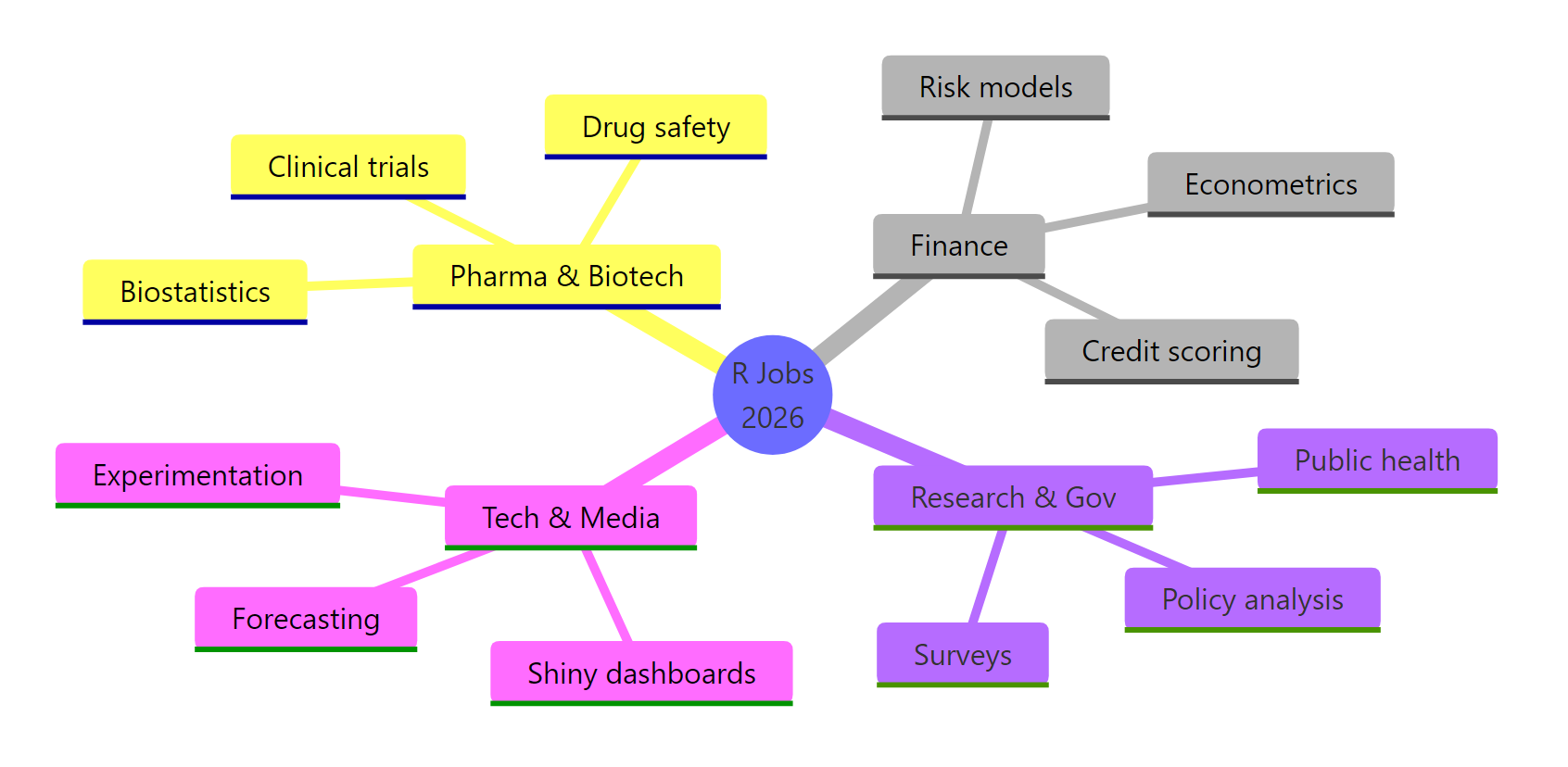
Industries where R dominates data-science hiring.

Figure 1: Where R is the dominant language, based on 2026 job-listing scans and Stack Overflow Developer Survey responses.

Let's put numbers to the picture. The tibble below rates each industry on two things: the median Senior-level pay and an R_share score that estimates the fraction of data-science roles where R is the primary tool.

RR-share and salary by industry

industries <- tribble( ~industry, ~median_senior_k, ~R_share, "Pharma & Biotech", 165, 0.62, "Clinical Research Orgs", 148, 0.71, "Finance & Banking", 175, 0.38, "Insurance & Actuarial", 152, 0.55, "Government & Public Health", 135, 0.58, "Academic & Research", 118, 0.66, "Tech & Software", 185, 0.22, "Media & Marketing", 140, 0.28, "Consulting", 160, 0.33 ) industries |> arrange(desc(R_share)) |> mutate(R_share = scales::percent(R_share, accuracy = 1)) #> # A tibble: 9 × 3 #> industry median_senior_k R_share #> <chr> <dbl> <chr> #> 1 Clinical Research Orgs 148 71% #> 2 Academic & Research 118 66% #> 3 Pharma & Biotech 165 62% #> 4 Government & Public Health 135 58% #> 5 Insurance & Actuarial 152 55% #> 6 Finance & Banking 175 38% #> 7 Consulting 160 33% #> 8 Media & Marketing 140 28% #> 9 Tech & Software 185 22%

Clinical Research Orgs (CROs) and Pharma are where R is genuinely dominant -- close to two-thirds of openings specify R as primary. Tech pays more, but R is a second-class citizen there, so you're competing against Python specialists on their home turf. Pick your battleground before you pick your stack.

Now let's isolate the roles where R gives you the biggest leg up -- industries with at least 55% R share.

RFilter R-dominant industries

r_heavy <- industries |> filter(R_share >= 0.55) |> arrange(desc(median_senior_k)) r_heavy #> # A tibble: 5 × 3 #> industry median_senior_k R_share #> <chr> <dbl> <dbl> #> 1 Pharma & Biotech 165 0.62 #> 2 Insurance & Actuarial 152 0.55 #> 3 Clinical Research Orgs 148 0.71 #> 4 Government & Public Health 135 0.58 #> 5 Academic & Research 118 0.66

Five industries clear the 55% bar, and they span a $47k spread at the Senior level. Pharma and Biotech lead on pay and R usage -- if you want the easiest path to a six-figure R role, that's the target. Academic pays 30-40% less but often gives 20% of your time to your own research, which is the implicit compensation.

Tip

Biotech and pharma hire R specialists year-round, not just during hiring seasons. The clinical-trial cycle runs 12 months, so there is always a team ramping up. Tech hiring freezes in Q4; pharma hiring doesn't. Factor that into when you start applying.

Try it: From industries, keep only rows where R_share > 0.5, then arrange by median_senior_k descending. Save the result to ex_r_dominant.

RExercise: filter R-dominant sectors

# Try it: filter + arrange ex_industries <- industries ex_r_dominant <- NA # your code here ex_r_dominant #> Expected: 5 rows, all R-dominant sectors, Pharma on top

Click to reveal solution

RR-dominant solution

ex_r_dominant <- ex_industries |> filter(R_share > 0.5) |> arrange(desc(median_senior_k)) ex_r_dominant #> # A tibble: 5 × 3 #> industry median_senior_k R_share #> <chr> <dbl> <dbl> #> 1 Pharma & Biotech 165 0.62 #> 2 Insurance & Actuarial 152 0.55 #> 3 Clinical Research Orgs 148 0.71 #> 4 Government & Public Health 135 0.58 #> 5 Academic & Research 118 0.66

Explanation: filter(R_share > 0.5) drops Finance (0.38), Consulting (0.33), Media (0.28), and Tech (0.22). arrange(desc(...)) sorts by the first column listed.

What skills do employers actually want at each career level?

"Proficient in R" on a resume fails the first ATS filter. Employers don't search for the language; they search for the packages, the statistical methods, and the deployment pattern they need on the team. The concrete skill names differ at every level, so let's map them out as a matrix instead of a list.

RSkills importance by career level

library(tidyr) skills_long <- tribble( ~skill, ~Junior, ~Mid, ~Senior, ~Staff, "dplyr / tidyr", 5, 5, 4, 3, "ggplot2 + themes", 4, 5, 4, 3, "Statistical modelling", 3, 5, 5, 5, "Shiny app deployment", 2, 4, 5, 4, "SQL + database joins", 4, 5, 5, 4, "Git + PR review", 3, 5, 5, 5, "R package authoring", 1, 3, 5, 5, "Cross-team communication", 2, 4, 5, 5, "Mentoring / hiring", 0, 1, 3, 5, "Infra + cloud (Docker, AWS)", 1, 3, 4, 5 ) |> pivot_longer( cols = Junior:Staff, names_to = "level", values_to = "importance" ) skills_long |> filter(skill == "Shiny app deployment") #> # A tibble: 4 × 3 #> skill level importance #> <chr> <chr> <dbl> #> 1 Shiny app deployment Junior 2 #> 2 Shiny app deployment Mid 4 #> 3 Shiny app deployment Senior 5 #> 4 Shiny app deployment Staff 4

The matrix uses a 0-5 importance score per skill per level, where 5 means "this is a hard filter -- you won't pass screening without it." The first five skills are table stakes at every level from Mid upward; the last three (package authoring, cross-team work, infra) are what separates Senior from Mid. Notice that pure coding skill peaks at Mid -- beyond that, impact skills dominate the scorecard.

Let's pull out exactly what a Senior candidate is being measured on.

RSenior must-have skills

senior_skills <- skills_long |> filter(level == "Senior", importance >= 4) |> arrange(desc(importance)) |> select(skill, importance) senior_skills #> # A tibble: 8 × 2 #> skill importance #> <chr> <dbl> #> 1 Statistical modelling 5 #> 2 Shiny app deployment 5 #> 3 SQL + database joins 5 #> 4 Git + PR review 5 #> 5 R package authoring 5 #> 6 Cross-team communication 5 #> 7 dplyr / tidyr 4 #> 8 ggplot2 + themes 4

Eight skills score 4 or 5 for a Senior R data scientist. Notice that "R package authoring" is a hard filter at Senior -- if you've never submitted to CRAN or at least shipped an internal package with tests, you're not competitive. The good news: it's a week of focused work to close that gap, not a year.

Warning

"Proficient in R" is resume poison. ATS systems search for package names, not languages. Replace the phrase with "dplyr, tidyr, ggplot2, Shiny, targets, testthat" and you'll clear 10x more filters. Name-dropping the ecosystem also signals that you ship real code, not just class assignments.

Try it: Find the skills that are already important at the Junior level -- importance ≥ 4. Save to ex_junior_skills.

RExercise: junior must-have skills

# Try it: Junior-level must-have skills ex_skills <- skills_long ex_junior_skills <- NA # your code here ex_junior_skills #> Expected: dplyr/tidyr and SQL, both with importance 4+

Click to reveal solution

RJunior-skills solution

ex_junior_skills <- ex_skills |> filter(level == "Junior", importance >= 4) |> select(skill, importance) ex_junior_skills #> # A tibble: 3 × 2 #> skill importance #> <chr> <dbl> #> 1 dplyr / tidyr 5 #> 2 ggplot2 + themes 4 #> 3 SQL + database joins 4

Explanation: Junior interviewers screen for the basic tidyverse trio plus SQL. Everything else on your resume is bonus at that level.

What does the career progression look like from junior to senior?

The typical R data science arc is 6-8 years from first job to Senior title, but the shape of the progression matters more than the length. Some people stall at Mid for five years; others skip the Junior band entirely with a strong PhD. Here's the visual map and then a cash-flow view.

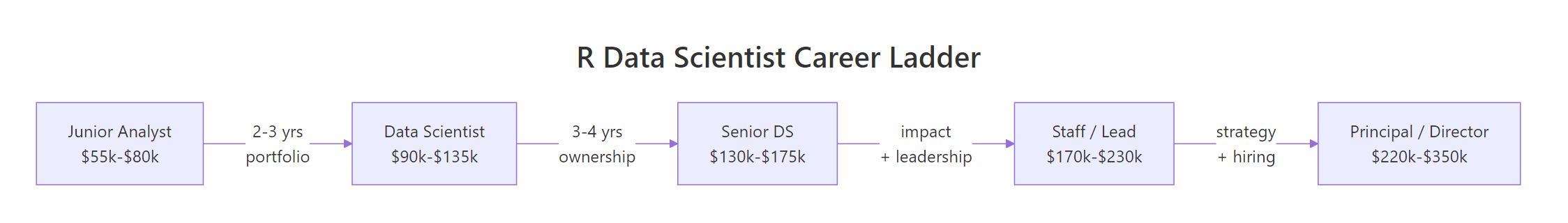
The typical R data scientist career ladder with salary bands.

Figure 2: The typical career ladder. Arrows show the common triggers for promotion at each level.

Each arrow is a promotion gate. Junior-to-Mid is gated on portfolio quality: can you ship a project end-to-end without someone holding your hand? Mid-to-Senior is gated on ownership: have you owned a metric that a VP cares about? Senior-to-Staff is gated on leadership: have you made other people on the team noticeably better? The gates change even when the language doesn't.

Now let's convert the ladder to real money over a realistic 10-year span -- assuming a typical 2-3-3-2 year cadence through the levels.

RCumulative earnings at each level

career_earn <- salaries |> mutate( years_at_level = c(2, 3, 3, 2, 0), level_total_k = mid_k * years_at_level ) |> select(level, mid_k, years_at_level, level_total_k) career_earn #> # A tibble: 5 × 4 #> level mid_k years_at_level level_total_k #> <chr> <dbl> <dbl> <dbl> #> 1 Junior 68 2 136 #> 2 Mid 112 3 336 #> 3 Senior 152 3 456 #> 4 Staff 200 2 400 #> 5 Principal 285 0 0 # Cumulative earnings over 10 years (pre-tax, pre-bonus) sum(career_earn$level_total_k) #> [1] 1328

$1.328 million in gross earnings over 10 years -- and that is before bonuses, equity, and the real value of the compounding raises in year 11+. Stall for an extra year at Junior and you lose roughly $44k from the total. Stall for two extra years at Mid and you lose $80k. The meta-lesson: promotions are the highest-leverage optimisation in the entire career, not side projects.

Note

This arc is faster in tech and slower in academia and government. A promising R engineer at a well-funded startup can hit Senior in 4 years; the same person at a federal lab might take 10. Neither is objectively better -- the trade is speed vs. stability vs. research freedom.

Try it: Recompute cumulative earnings assuming the reader stays 4 years at Mid instead of 3. Save the total to ex_slower_total.

RExercise: slower career climb

# Try it: slower climb, more time at Mid ex_earn <- salaries |> mutate(years_at_level = c(2, 4, 3, 2, 0), level_total_k = mid_k * years_at_level) ex_slower_total <- NA # your code here ex_slower_total #> Expected: 1440

Click to reveal solution

RSlower-climb solution

ex_slower_total <- sum(ex_earn$level_total_k) ex_slower_total #> [1] 1440

Explanation: An extra year at Mid adds 1 × $112k = $112k, so the 11-year total reaches $1.44M. The catch: you also delay every promotion downstream, which the tibble does not model.

How do I build a portfolio that gets R data scientist interviews?

Hiring managers don't read your resume first -- they read your GitHub. A portfolio that gets interviews has five ingredients, and you can grade any project against them. Let's build the scorecard as an R function so you can run it on your own work before submitting your next application.

RPortfolio scoring function

portfolio_score <- function(has_shiny_app = FALSE, has_package = FALSE, has_readme = FALSE, has_tests = FALSE, has_real_dataset = FALSE) { checks <- c( Shiny = has_shiny_app * 3, # highest weight Package = has_package * 2, README = has_readme * 2, Tests = has_tests * 2, RealDataset = has_real_dataset * 1 ) total <- sum(checks) verdict <- dplyr::case_when( total >= 8 ~ "Interview-ready", total >= 5 ~ "Promising -- add one more signal", total >= 3 ~ "Starter portfolio -- ship more", TRUE ~ "Not yet competitive" ) list(total = total, verdict = verdict, checks = checks) } my_checks <- portfolio_score( has_shiny_app = TRUE, has_package = FALSE, has_readme = TRUE, has_tests = TRUE, has_real_dataset = TRUE ) my_checks #> $total #> [1] 8 #> #> $verdict #> [1] "Interview-ready" #> #> $checks #> Shiny Package README Tests RealDataset #> 3 0 2 2 1

The function weights a deployed Shiny app highest because it proves three things at once: you can code, you can think about users, and you can deploy. A portfolio with a Shiny app, a README, tests, and a real dataset hits 8 points -- our "interview-ready" threshold. Notice that the CRAN-style package is worth 2 points but not required to clear the bar: ship the Shiny app first, then come back for the package.

Tip

One deployed Shiny app outweighs five Kaggle notebooks on a resume. Kaggle notebooks prove you can follow a tutorial. A deployed Shiny app proves you can handle state, user input, and production constraints -- which is what the job actually looks like.

Try it: Score a sample portfolio that has a Shiny app and a README but no tests, no package, and no real dataset. Save the result to ex_my_score.

RExercise: score a portfolio

# Try it: score a starter portfolio ex_my_score <- NA # call portfolio_score() with the right flags ex_my_score$total #> Expected: 5 ex_my_score$verdict #> Expected: "Promising -- add one more signal"

Click to reveal solution

RPortfolio-score solution

ex_my_score <- portfolio_score( has_shiny_app = TRUE, has_package = FALSE, has_readme = TRUE, has_tests = FALSE, has_real_dataset = FALSE ) ex_my_score$total #> [1] 5 ex_my_score$verdict #> [1] "Promising -- add one more signal"

Explanation: Shiny (3) + README (2) = 5 points. Adding tests would push you to 7; adding a real dataset would push you to 8 and into interview-ready territory.

Practice Exercises

These capstone exercises combine what you learned above. Both reuse the salaries and industries tibbles already in your session. Use distinct variable names (my_*) so you don't overwrite the teaching data.

Exercise 1: Highest-paying R-dominant industry at Senior

Join the idea of "R-dominant" (R_share >= 0.5) with the Senior-level pay column from industries. Find the single industry with the highest median_senior_k among R-dominant sectors and save its name to my_top_industry.

RExercise: top R-dominant industry

# Exercise 1: highest-paying R-dominant industry at Senior # Hint: filter, then slice_max() on median_senior_k my_top_industry <- NA my_top_industry #> Expected: "Pharma & Biotech"

Click to reveal solution

RTop-industry solution

my_top_industry <- industries |> filter(R_share >= 0.5) |> slice_max(median_senior_k, n = 1) |> pull(industry) my_top_industry #> [1] "Pharma & Biotech"

Explanation: slice_max(median_senior_k, n = 1) returns the single row with the highest median_senior_k. pull() extracts it as a plain character.

Exercise 2: Build a negotiation floor function

Write negotiation_floor(level, location_mult) that returns the 40th percentile of the band for that level, multiplied by location_mult. Assume the 40th percentile sits 40% of the way from low_k to high_k. Test it on Senior in NYC (multiplier 1.25) -- you should see roughly $185,000.

RExercise: negotiationfloor function

# Exercise 2: negotiation_floor() # Hint: look up the level's low_k and high_k in salaries, # compute low_k + 0.4 * (high_k - low_k), then multiply. negotiation_floor <- function(level, location_mult) { # your code here } negotiation_floor("Senior", 1.25) #> Expected: ~185 (k)

Click to reveal solution

Rnegotiationfloor solution

negotiation_floor <- function(level, location_mult) { row <- salaries |> filter(level == !!level) floor_k <- row$low_k + 0.4 * (row$high_k - row$low_k) round(floor_k * location_mult, 1) } negotiation_floor("Senior", 1.25) #> [1] 185 negotiation_floor("Mid", 0.9) #> [1] 97.2

Explanation: The !!level bang-bang unquotes the argument so dplyr doesn't confuse the argument with the column of the same name. The 40th percentile is conservative: it's what you should walk in with as your minimum acceptable offer, not your target.

Putting It All Together

A complete salary analysis in about 20 lines of R. This ties every previous block into one pipeline: take the raw bands, add cumulative earnings, join industry context, and plot the result with ggplot2.

RPlot the full salary ladder

library(ggplot2) career_plot <- salaries |> mutate( years_at_level = c(2, 3, 3, 2, 0), level = factor(level, levels = level) ) |> ggplot(aes(x = level, y = mid_k, fill = level)) + geom_col(show.legend = FALSE, width = 0.65) + geom_text(aes(label = paste0("$", mid_k, "k")), vjust = -0.4, size = 4) + scale_y_continuous(limits = c(0, 320)) + labs( title = "R data scientist median pay by level (2026, US)", subtitle = "Sources: Glassdoor, Levels.fyi, LinkedIn, BLS", x = NULL, y = "Median base pay ($k)" ) + theme_minimal(base_size = 12) career_plot

This block takes the same salaries tibble from earlier and produces a publication-ready plot. Notice how the pipeline flows: mutate() to lock the factor order so the bars don't re-sort alphabetically, geom_col() for the bars, geom_text() for the dollar labels, and theme_minimal() for a clean look. Swap mid_k for high_k to plot the ceiling of each band, or filter out Principal to match your realistic 10-year horizon.

Summary

Question	Answer
Typical starting salary (Junior, US)	$55k-$80k, median $68k
Senior median (6 years in)	$152k
Biggest percentage raise	Junior → Mid (~65%)
Most R-dominant industries	Pharma, Clinical Research, Academia
Highest-paying R-heavy sector	Pharma & Biotech ($165k median at Senior)
Top signal for a Junior portfolio	A deployed Shiny app + README + tests
Resume anti-pattern	"Proficient in R" with no packages named
Best single career move	Shipping the project that clears the Junior gate

References

U.S. Bureau of Labor Statistics -- Data Scientists occupational outlook. Link
Stack Overflow Developer Survey 2024 -- Languages used by data scientists. Link
Glassdoor -- R Programmer salary trends. Link
Levels.fyi -- Data Scientist compensation by level. Link
Burtch Works -- Data Science & Predictive Analytics Salary Report. Link
posit.co blog -- R in Industry case studies. Link
Kaggle State of Data Science 2023 -- Tool usage breakdown. Link

Continue Learning

Is R Worth Learning in 2026? -- The honest case for R today, including who should pick it over Python.
50 R Interview Questions Answered -- The exact technical questions you'll face going from Junior to Senior.
Best R Books: A Curated Reading List -- The 8 books that actually move the needle on R skill, ranked honestly.

R Data Scientist Salary & Career Path : Real Numbers, Real Requirements

How much do R data scientists actually earn in 2026?

Which industries hire the most R data scientists?

What skills do employers actually want at each career level?

What does the career progression look like from junior to senior?

How do I build a portfolio that gets R data scientist interviews?

Practice Exercises

Exercise 1: Highest-paying R-dominant industry at Senior

Exercise 2: Build a negotiation floor function

Putting It All Together

Summary

References

Continue Learning

Related Tutorials